9 Probability distributions for biologists
9.1 Introduction
All data contain some element of randomness. Understanding the nature and consequences of that randomness is what motivates much of modern statistics. Probability distributions are the mathematical constructs that describe randomness in data. This module describes some probability distributions commonly encountered in biology (and a few that aren’t common). The emphasis here is on practical understanding of what the distributions imply about data–not on the theoretical underpinnings or mathematical details. If you want or need a rigorous introduction to probability theory, this is probably not the right place.
9.1.1 Residuals: the random variation left over
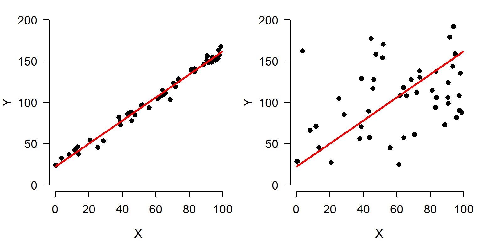
Consider the figures below:
Both scatterplots show a linear relationship between X and Y. But what is different about the plot on the right? Variation. Both plots show the same relationship (\(Y=22+1.4X\)), but they differ in that the variation about the expected value (the red line) is much greater in the right plot than the left plot. Consequently, X appears to explain much more variation in Y in the left plot than in the right plot. The next figure shows that the residual variation, or difference between the expected and observed values, is much greater in the right panel. Each of these differences between the observed value of Y (\(Y_i\)) and the expected value of Y (\(E(Y_i)\)), or \(Y_i-E(Y_i)\), is called a residual.
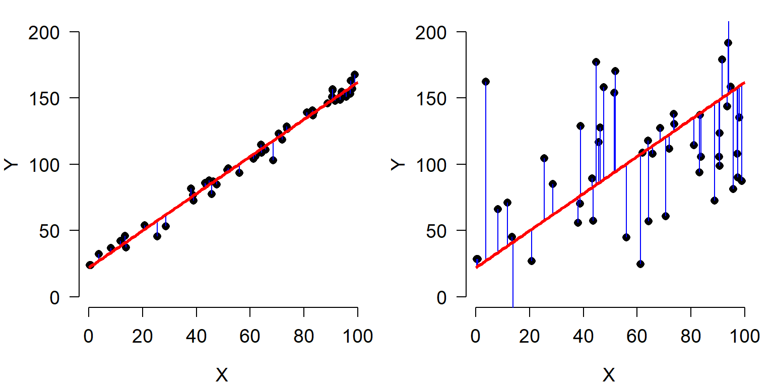
Residuals are an important part of statistical analysis for two reasons. First, most statistical models make assumptions about the distribution of residuals. Second, the total magnitude of the residuals (usually expressed as sum of squared residuals) is useful for calculating many measures of how well a model fits the data. The residuals of a statistical model are the differences between the observed values and the values predicted by the model. The residual for observation i in variable Y, \(R_i\), is calculated as:
\[R_i=Y_i-E\left[Y_i\right]\]
where \(E(Y_i)\) is the expected value of \(Y_i\). This means that when an observation has a greater value than predicted, the residual is positive; similarly, when an observation is smaller than expected, the residual is negative. In many statistical methods, residuals are squared so that (1) positive and negative residuals do not cancel out; and (2) larger residuals carry more weight.
The figures below show the distributions of residuals for the example linear regressions above. Notice that the left dataset has a much smaller distribution of residuals than the right dataset. This is because of the much tighter fit of the left dataset’s Y values to the predicted curve.
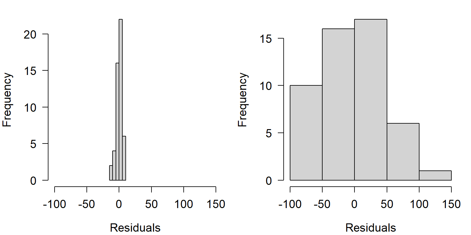
Notice also that both distributions of residuals have a similar shape, despite the difference in width. This shape is actually very important: the normal distribution. If the residuals were not distributed this way (i.e., did not follow a normal distribution), then we would be in trouble for two reasons. First, the data were generated using a normal distribution for residuals, so something would have had to have gone wrong with our statistical test; and second, the linear regression model used to analyze the data assumes that residuals are normally distributed. If they are not, then the test is not going to produce valid estimates of statistical significance or model parameters.
The example above is an example of the importance of thinking about statistical distributions when analyzing data. So just what is a statistical distribution? Distributions are mathematical functions that define the probabilities of random outcomes. Here random means that there is some element of chance in what we observe. This randomness is not completely unpredictable. While the outcome of specific observations might be unknowable, we can make predictions about long run frequencies or averages of lots of observations. In other words, single observations are not predictable, but the properties of sets of observations are. Such properties might include the number of times a specific outcome occurs (e.g., number of times a flipped coin comes up heads) or some summary of observations (e.g., the mean tail length of chipmunks). Another term for this kind of randomness that follows a pattern is stochastic.
Another example: coin flips
Consider flipping a coin. A fair coin will come up heads 50% of the time, and tails the other 50%. If you flip a coin once, the probability of getting heads is 50%. But what about if you flip the coin 10 times? How many heads should you get? 5 is a reasonable guess. The table below shows the possible outcomes to 10 coin flips:
| Heads | Tails |
|---|---|
| 0 | 10 |
| 1 | 9 |
| 2 | 8 |
| 3 | 7 |
| 4 | 6 |
| 5 | 5 |
| 6 | 4 |
| 7 | 3 |
| 8 | 2 |
| 9 | 1 |
| 10 | 0 |
This table shows that 5 heads is only one of 11 possibilities! So, is the probability of 5 heads 1 in 11 (\(1/11\approx0.091\))? Of course not, because not all outcomes are equally likely.
One of the reasons statistics is so fun is that we can often use simulation to discover patterns. The R code below will simulate the effects of flipping 1 coin 10 times. Run this code a few times and see what happens.
rbinom(1,10,0.5)[1] 4A typical run of results might be something like 4 5 5 4 3 5 6 6 5 5 4 6. We can repeat this line many times and graph the results:
x <- numeric(20)
for(i in 1:20){x[i] <- rbinom(1,10,0.5)}
plot(table(x))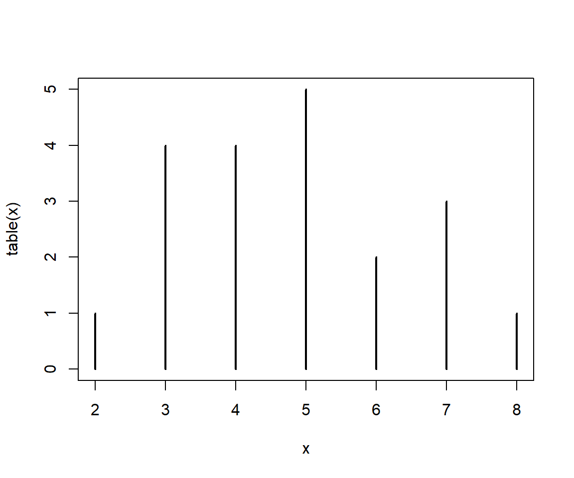
There is actually a faster way, by requesting 20 draws of 10 flips each all at once:
x <- rbinom(20,10,0.5)
plot(table(x))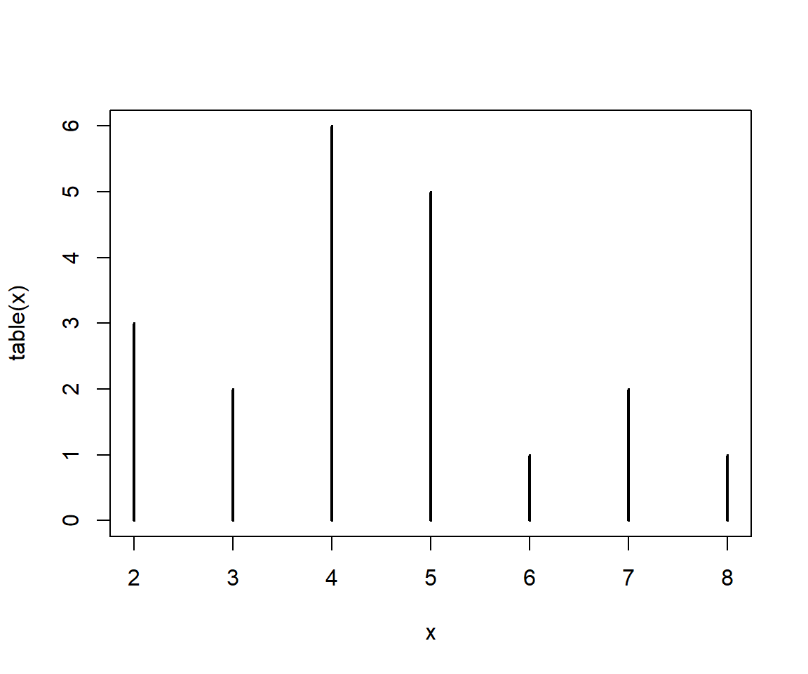
Is 5 the most likely value? What about if we get a larger sample?
x1 <- table(rbinom(10,10,0.5))
x2 <- table(rbinom(100,10,0.5))
x3 <- table(rbinom(1000,10,0.5))
x4 <- table(rbinom(10000,10,0.5))
x5 <- table(rbinom(100000,10,0.5))
x6 <- table(rbinom(1000000,10,0.5))

par(mfrow=c(2,3))
plot(x1, xlim=c(0, 10), main="n = 10")
plot(x2, xlim=c(0, 10), main="n = 100")
plot(x3, xlim=c(0, 10), main="n = 1000")
plot(x4, xlim=c(0, 10), main="n = 10000")
plot(x5, xlim=c(0, 10), main="n = 100000")
plot(x6, xlim=c(0, 10), main="n = 1000000")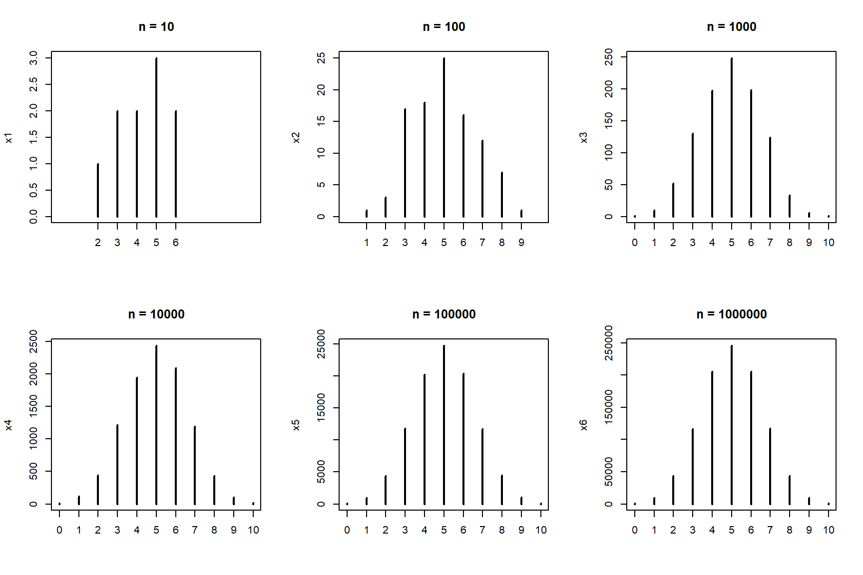
# reset graphical parameters
par(mfrow=c(1,1))
You may have guessed by now that the properties of a set of coin flips—such as what number of heads to expect—are described by some kind of mathematical function. This function is called a probability distribution. This particular distribution is the binomial distribution, which describes the outcome of any random process with a binary outcome. The name “binomial” is descriptive: “bi” for two, and “nomial” for names or states. Can you think of a biological situation where the binomial distribution might apply?
The sections below describe some distributions commonly encountered in biology, and what kinds of processes give rise to them. It is important to be able to relate biological phenomena to statistical distributions, because the underlying nature of the randomness in some process can affect how we analyze that process statistically. Note that in this class we will focus on the practical applications of these distributions, rather than their mathematical derivations.
9.1.2 Probability distributions in R
Every distribution supported in R has four functions associated with it: r__(), q__(), d__(), and p__() , where __ is the name of the distribution (or an abbreviation). These 4 functions calculate different values defined by the distribution:
r__()draws random numbers from the distribution.p__()calculates the cumulative distribution function (CDF) at a given value. The reverse ofq__().d__()calculates the probability density function (PDF); i.e., the height of the density curve, or first derivative of the CDF.q__()calculates the value at a given quantile. The reverse ofp__().
The figure below shows these functions in relation to the PDF and CDF for a normal distribution.
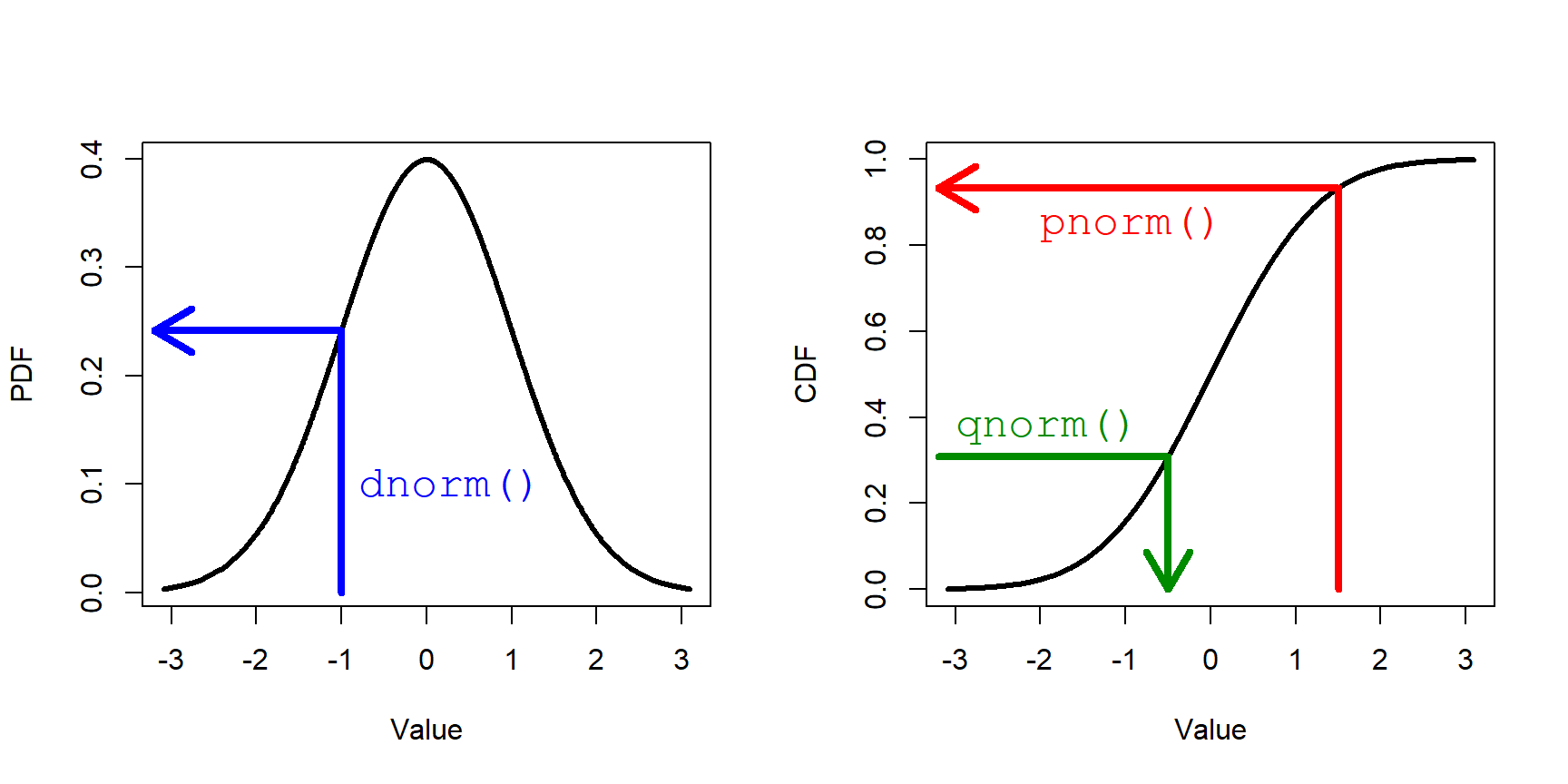
- If you want to know the value at the Xth percentile of a distribution, use the
q__function. - If you want to know the percentile of a value of a distribution, use the
p__function. - If you need to know the PDF of a distribution at some value, use the
d__function.
Here we see the functions used on a normal distribution with mean 20 and SD 4 (i.e., \(Normal\left(\mu=20,\sigma=4\right)\) or \(N\left(20,4\right)\)).
# 0.3 quantile (30th percentile)
qnorm(0.3, 20, 4)
[1] 17.9024# What value is at the 64th percentile? (0.64 quantile)?
pnorm(0.65, 20,4)[1] 6.574119e-07# What is the PDF at x == 23?
dnorm(23, 20, 4)[1] 0.07528436One use case might be drawing a CDF or PDF of a distribution manually to compare to your data or some other distribution. For example, here is how to draw the CDF of a normal with mean 10 and SD 2:
# values at which to draw CDF
xvals <- seq(0, 20, length=1000)

# distribution parameters
mu <- 10
sigma <- 2

# calculate CDF
xcdf <- pnorm(xvals, mu, sigma)

# make the plot
plot(xvals, xcdf, type="l", xlab="Value of x", ylab="CDF(x)")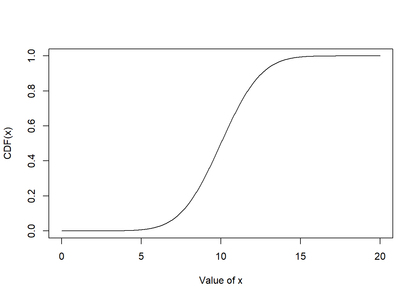
Here is how to draw the PDF of the same distribution:
# calculate CDF
xpdf <- dnorm(xvals, mu, sigma)

# make the plot
plot(xvals, xpdf, type="l", xlab="Value of x",
     ylab="Probability density of x")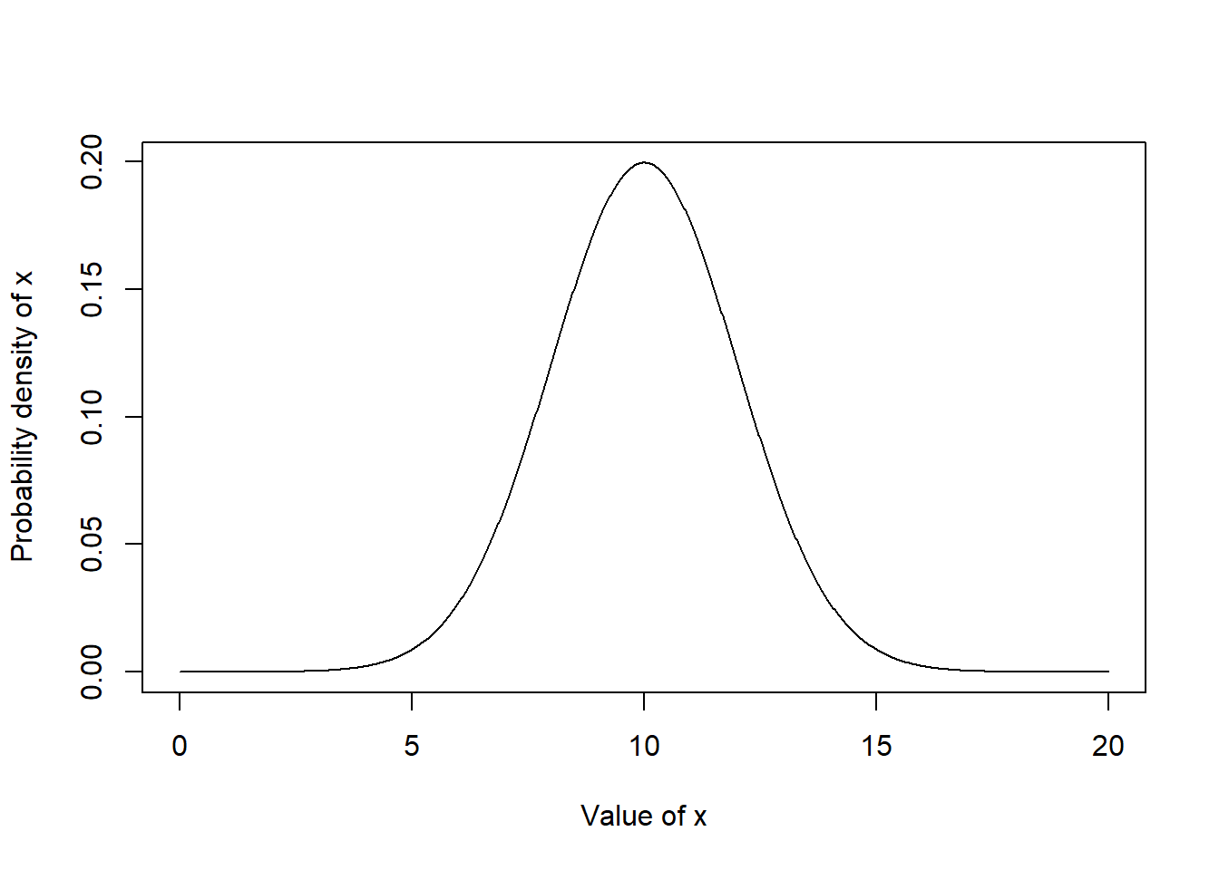
9.2 Discrete distributions
Discrete distributions can take on integer values only. Because of this, many discrete distributions are related in some way to count data. Count data result from, well, counting things. Count data can also describe the number of times something happened.
9.2.1 Bernoulli distribution
The simplest discrete distribution is the Bernoulli distribution. It describes the outcome of a single random event with probability p. Thus, the Bernoulli distribution takes the value 1 with probability p or the value 0 with probability \(q=\left(1-p\right)\). Any opportunity for the event to happen is also called a Bernoulli trial, and the process that it describes a Bernoulli process. The probability p can take on any value in the closed interval \(\left[0,1\right]\).
For convenience we usually consider a Bernoulli distribution to take the value of 0 or 1, but really it could represent any binary outcome. For example, yes vs. no, dead vs. alive, \(<3\) vs. \(\ge3\), etc., are all outcomes that could be modeled as Bernoulli variables. By convention, the event that occurs with probability p is considered a success and has the numerical value 1; the event that occurs with probability \(1-p\) is considered a failure and takes the numerical value 0. This is how Bernoulli variables are represented in most statistical packages, including R.
The Bernoulli distribution is rarely used on its own in an analysis. Instead, it’s useful to think of the Bernoulli distribution as a special case of, or a building block of, more complicated distributions such as the binomial distribution (Section 9.2.2). For example, a single observation of a binomially-distributed variable could be thought of as a Bernoulli distribution.
The Bernoulli distribution is a special case of the binomial distribution, and so it is accessed in R using the functions associated with the binomial. With the size argument set to 1, the binomial distribution is the Bernoulli distribution.
# flip one fair coin
rbinom(1, 1, 0.5)
[1] 0# flip 10 fair coins
rbinom(10, 1, 0.5) [1] 1 1 0 1 1 0 1 0 1 1# flip 10 coins with a 70% chance of heads
rbinom(10, 1, 0.7) [1] 0 1 1 0 1 1 0 0 0 19.2.2 Binomial distribution
The binomial distribution describes the number of successes in a set of independent Bernoulli trials. Each trial has probability of success p, and there are n trials. The values n and p are the parameters of the binomial distribution–the values that describe its behavior. The coin flipping example above is an example of a binomial distribution. Biological examples of binomial processes might be the number of fish that die in an experiment, or the number of plants that flower in a season. In such a case, the number of fish that start the experiment is the sample size n and the individual mortality rate is p.
Because it is so simple, thinking about the binomial distribution is a good warm up for learning about the characteristics of probability distributions. One of the most important characteristics is the expected value of the distribution. This is the value that most likely to occur, or the central tendency of values. There are several kinds of expected value, but they are all related to the most common or central value. The expected value, or mean, of a binomial distribution X is
\[E\left(x\right)=\mu=np\]
This is the answer to the question earlier about how many heads to expect if a fair coin is flipped 10 times:
\[E(heads)=n(flips)p(heads)\]
If a variable comes from a binomial process, we can make other inferences about it. For example, we can estimate its variance as:
\[Var\left(x\right)=\sigma^2=np(1-p)=npq\]
We can also estimate the probability of any number of successes k as:
\[P\left(k\right)=\left(\begin{matrix}n\\k\\\end{matrix}\right)p^k\left(1-p\right)^{n-k}\]
The first term (n over k) is known as the binomial coefficient and is calculated as:
\[\left(\begin{matrix}n\\k\\\end{matrix}\right)=\frac{n!}{k!\left(n-k\right)!}\]
This term represents the number of ways of seeing k successes in n trials. For example, a set of 4 trials could have 2 successes in 6 ways: HHTT, HTHT, THHT, HTTH, THTH, and TTHH.
When n is small, the binomial distribution can be quite skewed (i.e., asymmetric) because the distribution has a hard lower bound of 0. Note that the expression for \(P(k)\) is what is calculated by function dbinom() below, and related to what is calculated by function pbinom(). For large n, the binomial distribution can be approximated by a normal distribution1 with mean = np and variance = npq.
9.2.2.1 Binomial distribution in R
R uses a family of 4 functions to work with each probability distribution. The binomial and Bernoulli distributions are accessed using the _binom group of functions: dbinom(), pbinom(), qbinom(), and rbinom(). Each function calculates or returns something different about the binomial distribution:
dbinom(): Calculates probability mass function at x for binomial distribution given n and p. Answers the question “What is the probability of x successes in n trials with probability p?”pbinom(): Calculates integral of the probability mass function for a binomial distribution given n and p, from 0 up to x. In other words, given some binomial distribution, at what quantile of that distribution should some value fall? The reverse ofqbinom(). Answers the question “What is the probably of at least x successes in n trials with probability p?”qbinom(): Calculates the value at specified quantile of a binomial distribution. Essentially the reverse ofpbinom().rbinom(): Draws random numbers from the binomial distribution defined by n and p (or from the Bernoulli distribution if n = 1).
Let’s explore the binomial distribution using these functions. In the plots produced in the two examples, notice how the variance of each distribution (x1, x2, etc.) depends on both n and p. The variance in these plots is shown by the width of the distribution.
# N = 100, P various
N <- 100
X <- 0:100
x1 <- dbinom(X, N, 0.2)
x2 <- dbinom(X, N, 0.4)
x3 <- dbinom(X, N, 0.6)
x4 <- dbinom(X, N, 0.8)

par(mfrow=c(1,1))
plot(X, x1, pch=16, xlab="X", ylab="PMF")
points(X, x2, pch=16, col="red")
points(X, x3, pch=16, col="blue")
points(X, x4, pch=16, col="green")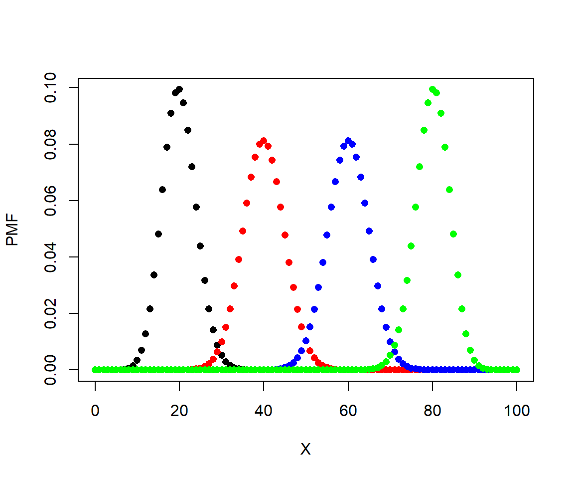
Here is a plot showing the effect of varying n.
# P = 0.5, N various
P <- 0.5
x1 <- dbinom(0:100, 20, P)
x2 <- dbinom(0:100, 40, P)
x3 <- dbinom(0:100, 60, P)
x4 <- dbinom(0:100, 80, P)
x5 <- dbinom(0:100, 100, P)

plot(0:100, x1, pch=16, xlab="X", ylab="PMF")
points(0:100, x2, pch=16, col="red")
points(0:100, x3, pch=16, col="blue")
points(0:100, x4, pch=16, col="green")
points(0:100, x5, pch=16, col="purple")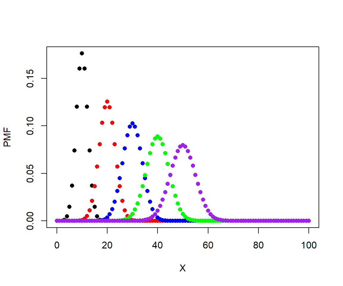
In these plots, the height of the points is called the probability mass function (PMF). For discrete distributions like the binomial, the PMF of any value is the probability that the distribution takes on that value. The sum of the PMF for all integers from 0 to n (inclusive) must be equal to 1. You can verify this by calculating the sum of any of the vectors of densities above.
The function pbinom() sums the PMF from 0 up to and including some value. In other words, it calculates the cumulative distribution function (CDF). This answers the question “where in the distribution is value x?”; put another way, “at what quantile of the distribution does value x lie?”. Yet another way to ask this is, “What is the probability of at least X successes?”.
Consider a binomial distribution with \(n=10\) and \(p=0.5\). What is the probability that the distribution takes a value \(\le7\)? We can calculate this as the sum of the PMF for 0 through 7.
# plot the distribution to see it
N <- 10
P <- 0.5
xd <- dbinom(0:10, N, P)
plot(0:10, xd, type="h", xlab="X", ylab="PMF")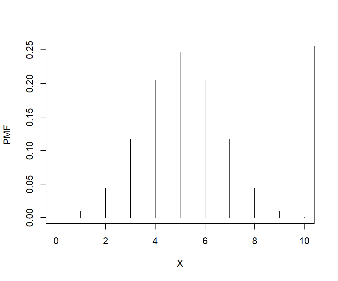
# calculate p(x<=7)
sum(xd[1:8]) # indices 1:8 correspond to values 0:7
[1] 0.9453125# same value:
pbinom(7, N, P)[1] 0.9453125Or, we could want to know the probability that the distribution takes on a value \(>6\). This would be the complement of the sum up to and including 6.
1-sum(xd[1:7])[1] 0.171875# same value:
1-pbinom(6,N,P)[1] 0.171875If the last two calculations seem familiar, that’s because this is exactly how p-values for statistical tests are calculated (e.g., using pf() to get the probability from an F distribution for an ANOVA).
The function qbinom() is basically the reverse of function pbinom(). Rather than calculate the quantile at which a value falls in the distribution, qbinom() calculates the value at which a quantile falls. For example, what value do we expect to find at the 60th percentile of a distribution? Put another way, how many successes should 60% of experiments have, on average? The example below shows how qbinom() and pbinom() are reversible.
N <- 10
P <- 0.5
pbinom(6, N, P)
[1] 0.828125# same value
qbinom(0.828125, N, P)[1] 6Finally, rbinom() draws random values from the binomial or Bernoulli distributions. The syntax of this function can be a little confusing. The first argument, n, is the number of random draws that you want. The second argument, size, is the number of values in each draw; that is, the parameter n of the binomial distribution. Compare these results, all with p = 0.5:
# 1 draw of 1 trial
rbinom(1, 1, 0.5)
[1] 0# 1 draw of 10 trials
rbinom(1, 10, 0.5)[1] 8# 10 draws of 1 trial per draw
rbinom(10, 1, 0.5) [1] 0 0 1 0 1 1 1 0 1 0# 10 draws of 10 trials per draw
rbinom(10, 10, 0.5) [1] 3 5 5 7 3 5 5 5 4 3- Result 1 shows a Bernoulli distribution with n = 1.
- Result 2 shows a single value from a binomial distribution with n = 10.
- Result 3 shows 10 results from Bernoulli distributions. Notice that if you add up the values in Result 3, you get a result like Result 2.
- Finally, Result 4 shows 10 draws from a binomial distribution, which itself has n = 10.
The take home message is that the first argument to rbinom() is not a parameter of the binomial distribution. It is instead the number of draws from the distribution that you want. The size parameter is the argument that helps define the distribution.
9.2.3 Poisson distribution
The Poisson distribution is widely used in biology to model count data. If your data result from some sort of count or abundance per time interval, spatial extent, or unit of effort, then the Poisson distribution should be one of the first things to try in the analysis. The Poisson distribution has one parameter, \(\lambda\) (“lambda”), which represents the expected number of objects counted in a sample (objects being trees, fish, cells, mutations, kangaroos, etc.). This parameter is also the variance of the distribution. This is a very important property, as we will see later: the expected value and the variance of the Poisson distribution are both \(\lambda\):
\[E\left(X\right)=Var\left(X\right)=\lambda\]
Like the binomial distribution, the Poisson distribution is discrete, meaning that it can only take on integer values. Unlike the binomial distribution, which is bounded by 0 and n, the Poisson distribution is bounded by 0 and \(+\infty\). However, values \(\gg \lambda\) are highly improbable. If there is a well-defined upper bound for your count, then you might consider them to come from a binomial model instead of a Poisson model. For example, if you are counting the number of fish in a toxicity trial that survive, the greatest possible count is the number of fish in the trial. This means that your “count” is really another way of representing a proportion. On the other hand, if your counts have no a priori upper bound, then use the Poisson.
9.2.3.1 Poisson distribution in R
The Poisson distribution is accessed using the _pois group of functions, where the space could be d, p, q, or r. These functions calculate or returns something different:
dpois(): Calculates probability mass function (PMF) at x for Poisson distribution given \(\lambda\). Answers the question, “what is the probability of observing a count of x given \(\lambda\)?”ppois(): Calculates CDF, or integral of PMF, from 0 up to x given \(\lambda\). In other words, given some Poisson distribution, at what quantile of that distribution should some value fall? The reverse ofqpois().qpois(): Calculates the value at specified quantile of a Poisson distribution. The reverse ofppois().rpois(): Draws random numbers from the Poisson distribution defined by \(\lambda\).
Something important to keep in mind about the Poisson distribution is that it only makes sense for discrete counts, not for continuous measurements that are rounded. For example, if you are measuring leaf lengths and round every length to the nearest mm, it might be tempting to use a Poisson distribution to analyze the data because all of the values are integers. But that would be incorrect, because leaf lengths could theoretically take on any positive value. Furthermore, treating rounded continuous values as discrete leads to the awkward issue that changing measurement units can change dimensionless statistics.
For example, the coefficient of variation (CV) is the ratio of a distribution’s SD to its mean. Thus, it is unitless and should be independent of units. The CV of a Poisson distribution X is:
\[CV\left(X\right)=\frac{\sqrt\lambda}{\lambda}\]
So, if you measured 20 leaves and found a mean length of 17 cm, the CV would thus be \(\approx\) 0.242 or 24%. But if you convert the measurements to mm, the CV would be about 0.077, or 7.7%!
The figure below shows the effect of varying \(\lambda\) on a Poisson distribution.
x <- 0:40
lams <- c(1,5, 10, 20)
nlams <- length(lams)
dlist <- vector("list", nlams)
for(i in 1:nlams){dlist[[i]] <- dpois(x, lams[i])}
cols <- rainbow(nlams)

par(mfrow=c(1,1), mar=c(5.1, 5.1, 1.1, 1.1),
    las=1, bty="n", lend=1,
    cex.lab=1.3, cex.axis=1.3)
plot(x, dlist[[1]], ylim=c(0, max(sapply(dlist, max))),
    type="n", ylab="PMF", xlab="Value (x)")
for(i in 1:nlams){
    points(x, dlist[[i]], pch=i, cex=1.3,
        col=cols[i])
}
legend("topright", legend=lams,
    pch=1:nlams, pt.cex=1.3, col=cols, bty="n", cex=1.3,
    title=expression(lambda))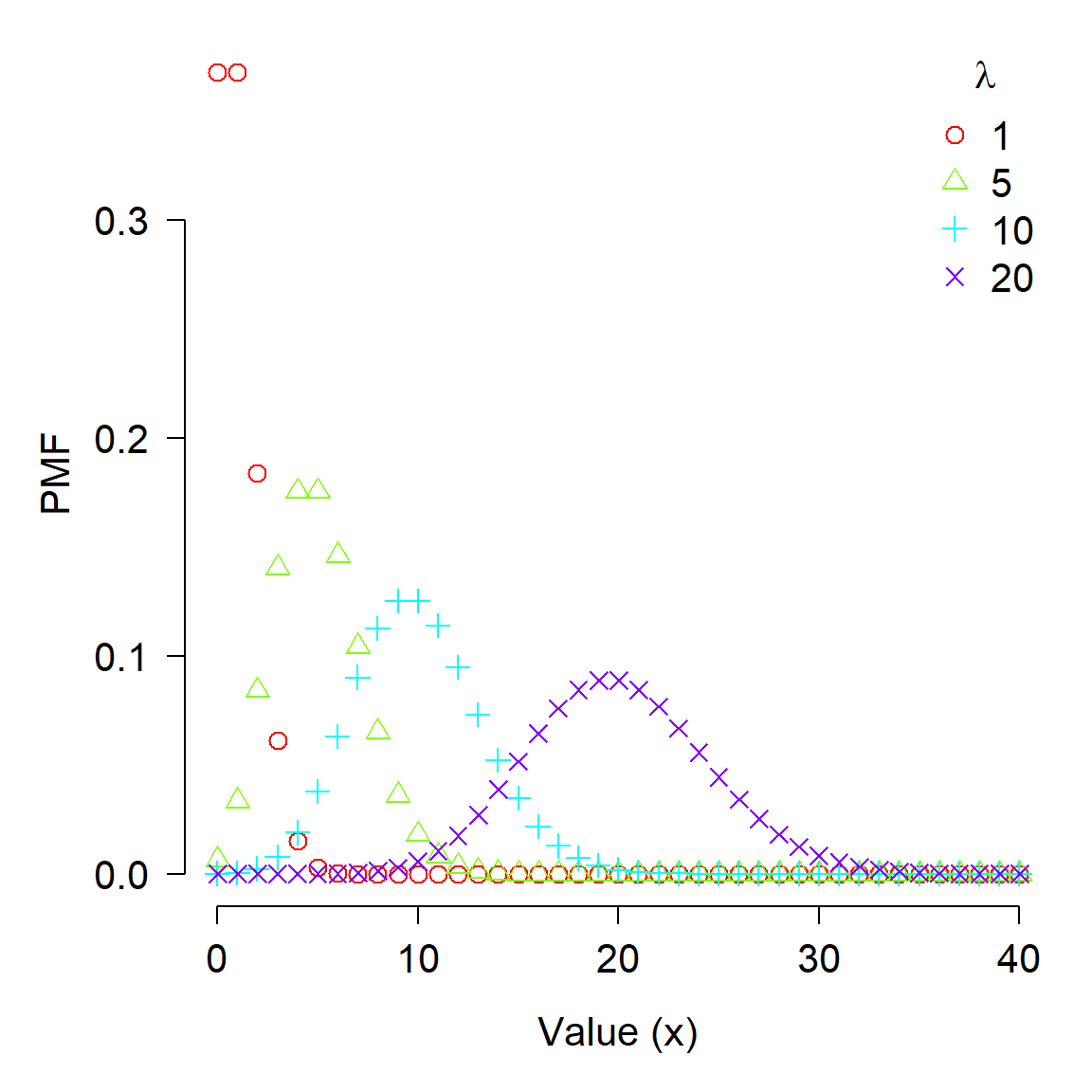
9.2.4 Negative binomial distribution
The negative binomial distribution as usually used in biology is used for counts that are overdispersed–that is, they have a variance greater than expected given other parameters. In this case, that means \(\sigma^2>>\lambda\). This is very common in biological count data. For example, a bird species might have low abundance (0 to 4) at most sites in a study, but very high abundance (30 to 40) at a handful of sites. In that case using the Poisson distribution would not be appropriate because doing so would mean assuming that the variance was approximately equal to the mean when it really wasn’t.
The definition that is not used as commonly in biology is actually the original definition: the negative binomial distribution also describes the number of failures that occur in a series of Bernoulli trials until some predetermined number of successes is observed. For example, when flipping a fair coin, how many times should you expect to see tails before you observe 8 heads? This definition is, therefore, a discrete version of the gamma distribution. This also makes the original definition of the negative binomial similar to the geometric distribution (Section 9.2.5).
The version of the negative binomial that biologists use is parameterized by its mean \(\mu\) and its overdispersion \(k\). This definition views the negative binomial as a Poisson distribution with parameter \(\lambda\), where \(\lambda\) itself is a random variable that follows a Gamma distribution (Section 9.3.4). For this reason, some authors refer to the negative binomial as a Gamma-Poisson mixture distribution. A mixture distribution is exactly what it sounds like: a distribution that is formed by “mixing” or combining two distributions. Often a mixture is formed by having parameters of one distribution vary according to another distribution.
The overdispersion parameter \(k\) is called size in the R functions that work with the negative binomial. Counterintuitively, the overdispersion in a negative binomial distribution gets larger as \(k\) becomes smaller. This is seen in the expression for the variance of a negative binomial distribution:
\[Var\left(X\right)=\mu+\frac{\mu^2}{k}\]
As \(k\) becomes large, the ratio \(\mu^2/k\) becomes small and approaches 0, and thus \(Var(x)\) approaches \(\mu\). This means that a negative binomial distribution with large \(k\) approximates a Poisson distribution. As \(k\) approaches 0, the ratio \(\mu^2/k\) becomes larger, and thus \(Var(x)\) increases to be much larger than \(\mu\).
9.2.4.1 Negative binomial distribution in R
The negative binomial distribution is accessed using the _nbinom group of functions, where the space could be d, p, q, or r. These functions calculate or returns something different:
dnbinom(): Calculates PMF at x. Answers the question, “what is the probability of observing a count of x?”pnbinom(): Calculates CDF, or integral of PMF, from 0 up to x. In other words, given some negative binomial distribution, at what quantile of that distribution should some value fall? The reverse ofqnbinom().qnbinom(): Calculates the value at specified quantile of a Poisson distribution. The reverse ofpnbinom().rnbinom(): Draws random numbers from the negative binomial distribution.
The R functions for the negative binomial distribution can work with either parameterization (waiting time or mean with overdispersion). Some of the argument names are used for both methods. If you are working with the negative binomial distribution in R you need to name your arguments to make sure you get the version of the negative binomial that you want.
The figure below shows the effect of different overdispersion parameters. Notice that as \(k\) increases, the distribution looks more and more like a Poisson distribution with \(\lambda = 10\). As \(k\) gets smaller, the distribution gets more and more concentrated near 0, and more and more right-skewed.
xp <- 0:30
y1 <- dpois(xp, 10)
y2 <- dnbinom(xp, size=0.2, mu=10)
y3 <- dnbinom(xp, size=0.5, mu=10)
y4 <- dnbinom(xp, size=1, mu=10)
y5 <- dnbinom(xp, size=10, mu=10)
y6 <- dnbinom(xp, size=50, mu=10)
y7 <- dnbinom(xp, size=100, mu=10)

cols <- rainbow(6)
par(mfrow=c(1,1), mar=c(5.1, 5.1, 1.1, 1.1),
    las=1, bty="n", lend=1,
    cex.lab=1.3, cex.axis=1.3)
plot(xp, y1, pch=17, ylim=c(0, 0.5), xlab="X", ylab="PMF")
points(xp, y2, pch=16, col=cols[1])
points(xp, y3, pch=16, col=cols[2])
points(xp, y4, pch=16, col=cols[3])
points(xp, y5, pch=16, col=cols[4])
points(xp, y6, pch=16, col=cols[5])
points(xp, y7, pch=16, col=cols[6])
legend("topright",
legend=c("Poisson", "k=0.2", "k=0.5", "k=1", "k=10",
"k=50", "k=100"),
     pch=c(17, rep(16,6)), col=c("black", cols))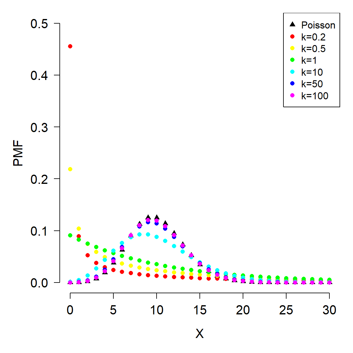
9.2.5 Geometric distribution
The geometric distribution describes the number of failures that are seen before observing the first success, given that the probability remains constant. It is thus related to the binomial and negative binomial. In fact, the geometric distribution is a special case of the negative binomial, with the number of successes = 1. The geometric distribution is the discrete version of the exponential distribution.
The geometric distribution arises in biology when modeling waiting times or life spans in discrete time steps. For example, if an animal has a constant annual mortality rate, the geometric distribution models the number of years that an individual organism completes before dying. Age- or stage-based population matrix models such as Leslie matrices are common in wildlife and fisheries management, and are based on annual monitoring data. So, it makes sense to use a discrete distribution to model survival in yearly time steps rather than continuous time. Another biological example of when to use a geometric distribution would be counting the number of generations until a mutation in a cell line occurs, if mutations occur at a constant rate per generation.
Imagine a fish that has a 5% probability of dying each year (i.e., a 95% annual survival rate). If \(X\) is the number of complete years the fish survives before dying, then \(X\) follows a geometric distribution with \(p=0.05\). Let’s simulate a cohort of 100,000 fish to see what this looks like.
# set annual mortality rate
P <- 0.05

# simulate 100000 fish
fish <- rgeom(1e5, P)

# plot the resulting lifespans
use.breaks <- seq(-0.5, max(fish)+0.5, by=1)
hist(fish, breaks=use.breaks, freq=FALSE, xlim=c(0, 80),
     xlab="Years survived before death")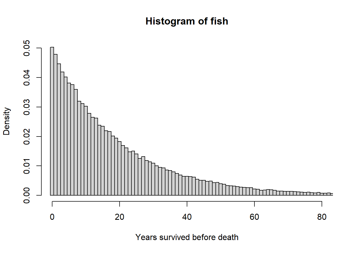
Notice that the distribution of simulated fish lifespans has a long right tail: there are many small values, and a few very large values. We also call this right skewed. Practically, this means that while the median lifespan is 13 years, the average fish lives to 19. The long tail pulls the arithmetic mean upwards.
# by what age do 50% of fish die?
median(fish)
[1] 13# how long does the "average" fish live?
mean(fish)[1] 19.07688Compare our simulation to the theoretical distribution:
X <- 0:max(fish)

pmf <- dgeom(X, P)
hist(fish, breaks=use.breaks, freq=FALSE, xlim=c(0, 80),
     xlab="Years survived before death",
     ylim=c(0, 0.05),
     main="Simulated vs. theoretical distribution")
points(X,pmf, type="s", lwd=2, col="red")
meanfish <- round(mean(fish),0)
segments(meanfish, 0, meanfish, dgeom(meanfish,P),
         lwd=2, col="blue")
# calculate theoretical mean - matches simulation
theomean <- (1-P)/P
segments(theomean, 0, theomean, dgeom(theomean,P),
         lwd=2, lty=2, col="black")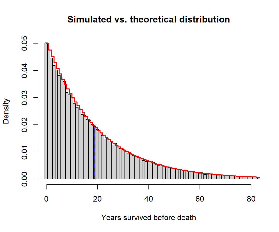
The figure shows that the probability of living to any given age falls off quickly at first, then more gradually as time goes on. We can also answer questions like “What is the probability that a fish lives to at least 30 years old?
# answer based on simulation
# off a bit because of sampling variation
length(which(fish >= 30)) / length(fish)
[1] 0.21554# answer based on distribution:
pgeom(29, P, lower.tail=FALSE)[1] 0.2146388Or equivalently:
(1-P)^30[1] 0.2146388What age will 95% of fish reach?
qgeom(0.95, P)[1] 589.2.6 Multinomial distribution
The multinomial distribution is a generalization of the binomial distribution to cases with more than 2 possible outcomes. For example, rolling a 6-sided die many times would yield a distribution of outcomes (1, 2, 3, 4, 5, or 6) described by the multinomial distribution. The multinomial distribution is parameterized by the number of possible outcomes k, the number of trials n, and the probabilities of each outcome \(p_1, \ldots, p_k\). The probabilities must sum to 1.
There are some special cases of the multinomial distribution:
- When \(k=2\) and \(n=1\), the multinomial distribution reduces to the Bernoulli distribution
- When \(k=2\) and \(n>1\), the multinomial distribution reduces to the binomial distribution
- When \(k>2\) and \(n=1\), the multinomial distribution is the categorical distribution.
The example below shows how to work with the multinomial distribution in R.
# define 2 different sets of probabilities for
# 5 different outcomes
p1 <- c(0.2, 0.2, 0.1, 0.1, 0.4)
p2 <- c(0.1, 0.2, 0.4, 0.2, 0.1)

# sample from the multinomial distribution
N <- 1e3
r1 <- rmultinom(N, N, prob=p1)
r2 <- rmultinom(N, N, prob=p2)

# summarize by outcome
y1 <- apply(r1, 1, mean)
y2 <- apply(r2, 1, mean)

# plot the results
plot(1:5, y1, pch=16, xlab="X",
     ylab="Frequency", ylim=c(0, 1000))
points(1:5, y2, pch=16, col="red")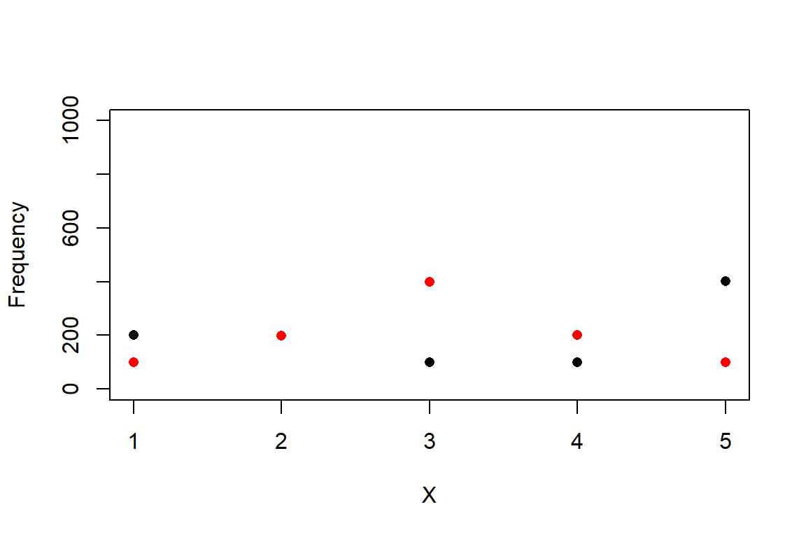
9.3 Continuous distributions
A continuous distribution can take on any real value within its supported interval. This means that unlike discrete distributions, continuous distributions are not restricted to integers. Measurements like length, mass, temperature, etc., are best modeled using continuous distributions because, although we often record them to the nearest mm, gram, or degree, the underlying quantity varies continuously. The apparent discreteness comes from the limited precision of our measuring instruments.
Computing the probability of any possible outcome of a discrete distribution is relative straightforward because there are a limited number of outcomes. For example, a binomial distribution with \(n=10\) and \(p=0.5\) has only 11 possible outcomes \(\left(0,1,2,\ldots,9,10\right)\). The probabilities \(p\left(x=0\right)\), \(p\left(x=1\right)\), and so on up to \(p\left(x=10\right)\) must all sum to 1. The probability mass function (PMF) of the binomial distribution at any value is the probability of that value occurring.
This leads to an interesting question. How could we calculate the probability of any given outcome of a distribution with an infinite number of outcomes? If the probabilities of each individual value must all sum to 1, and there are infinitely many possible values, then each individual value must have probability 0. If the probability of every possible outcome is 0, how can the distribution take on any value at all?
To resolve this apparent contradiction, we have to take a step back and think about what distributions really mean. The first step is to realize that even if any single value has probability 0, an interval of values can have a non-zero probability. After all, the entire supported interval of a distribution has probability 1 by definition. We can define some interval extending from the lower limit of the distribution up to some value \(x\). This means that for any value \(x\) in a distribution \(X\) (note lower case vs. upper case) we can calculate the probability of observing a value \(\le{x}\), or \(p\left(X\le{x}\right)\). The figure below shows this:
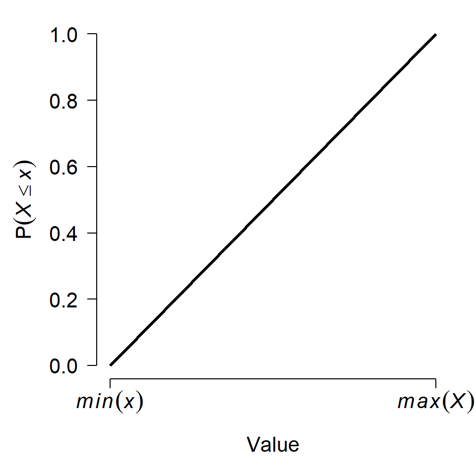
The y-axis in the figure, \(P\left(X\le{x}\right)\), is called the cumulative distribution function (CDF). This name derives from the fact that the CDF of some value \(x\) gives the cumulative or total probability of all values up to and including \(x\). The CDF is sometimes labeled \(F\left(x\right)\) (note the capitalized F). Another way to interpret this is that a value \(x\) lies at the \(CDF\left(x\right)\) quantile of a distribution. For example, if \(CDF\left(x\right)=0.4\), then \(x\) lies at the 0.4 quantile or 40th percentile of the distribution. Critically, this means that 40% of the total probability of the distribution lies at or to the left of \(x\), and the remaining 60% of the probability lies to the right of \(x\).
Just as the PMF describes how probability is distributed among the possible values of a discrete random variable, the probability density function PDF describes how probability is distributed over the continuum of possible values. Although the PDF is not itself a probability, the area under the PDF between any two values equals the probability that the random variable falls within that interval. Mathematically, the PDF is the rate at which the CDF changes with respect to \(x\). That is, the PDF, \(f\left(x\right)\), is the derivative of the CDF \(F\left(x\right)\) evaluated at \(x\):
\[f\left(x\right)=\frac{dF(x)}{dx}\]
This also means that the CDF is the integral of the PDF up to \(x\), according to the fundamental theorem of calculus:
\[F\left(x\right)=\int_{-\infty}^{x}{f\left(x\right)\ dx}\]
In other words, probabilities correspond to areas under the PDF, while the PDF itself represents the local density of probability. These areas under the PDF correspond to values of the CDF.
This might be easier to see with an example. The plots below show the PDF and CDF of a standard normal distribution with mean 0 and SD 1 (Section 9.3.2). Because the normal is unbounded, its PDF and CDF have the domain \([-\infty,+\infty]\), but we usually truncate the plot to a range that covers most of the CDF. For the normal, the mean plus or minus 3 standard deviations, or \(\mu\pm{3\sigma}\), covers over 99.7% of values.
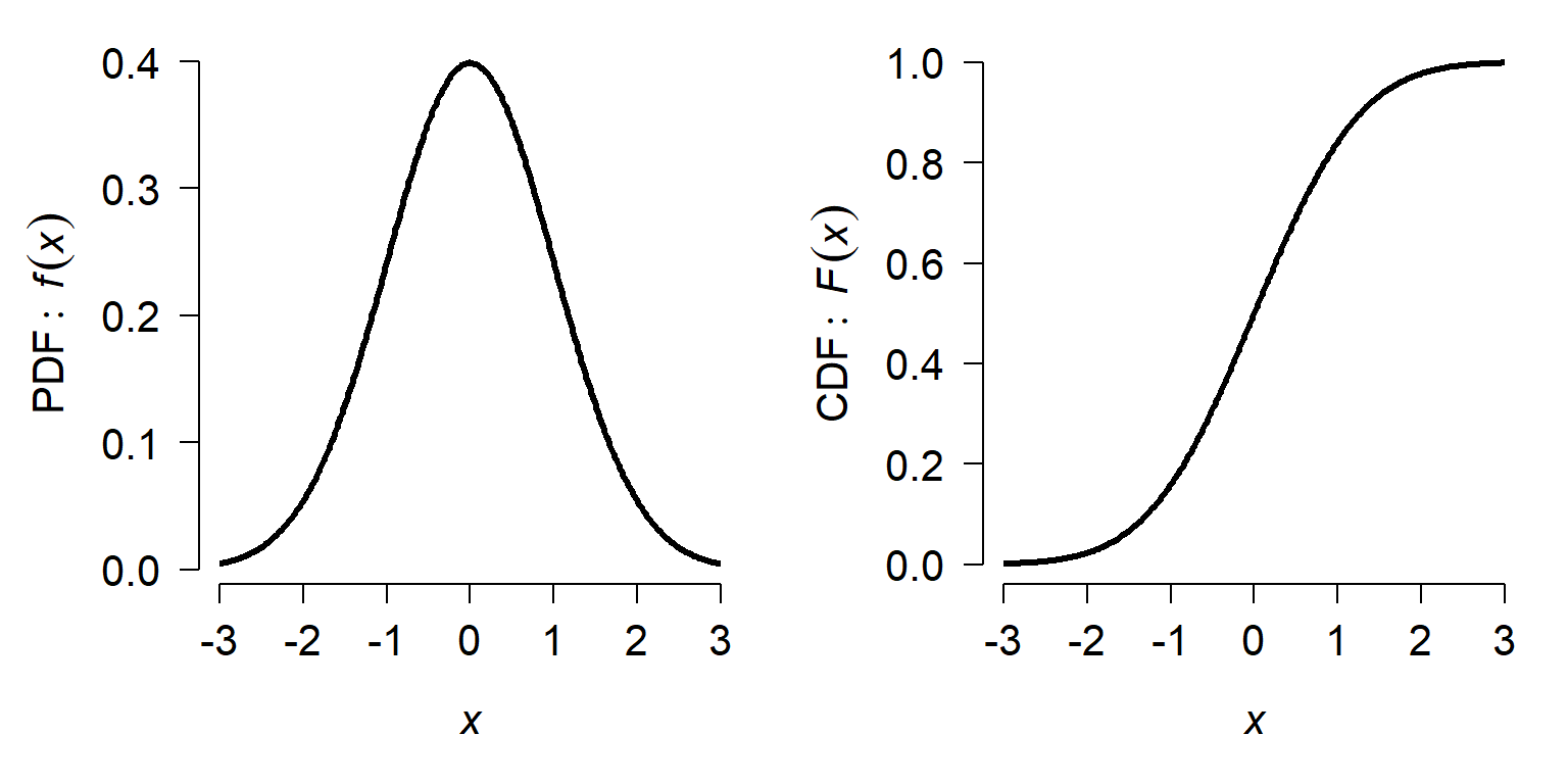
On the left, notice that the PDF peaks near \(x=0\) and tapers off quickly to either side. On the right, the slope of the CDF is greatest at \(x=0\). The value of the PDF at \(x=0\), about 0.4, is neither the probability of observing \(x=0\) (which is 0) nor the probability of observing \(x\le0\) (which is 0.5). The value \(f(0)=0.4\) is the rate of change or slope in \(F(X)\) at \(x=0\).
If we wanted to calculate something like the probability of \(x=0\), we would actually have to calculate the probability of \(x\) being in some interval that included 0. For example, the probability that \(-0.1\le{X}\le+0.1\), or that \(X\in\left[-1,+1\right]\), is
\[P\left(-0.1\le{X}\le+0.1\right)=F\left(0.1\right)-F\left(-0.1\right)\]
In R we can calculate:
pnorm(0.1)-pnorm(-0.1)[1] 0.07965567So the probability that \(x\) is within 0.1 of 0 is about 0.08 or 8%. If we use a narrow interval, say \(-0.01\le{X}\le+0.01\), the calculation becomes:
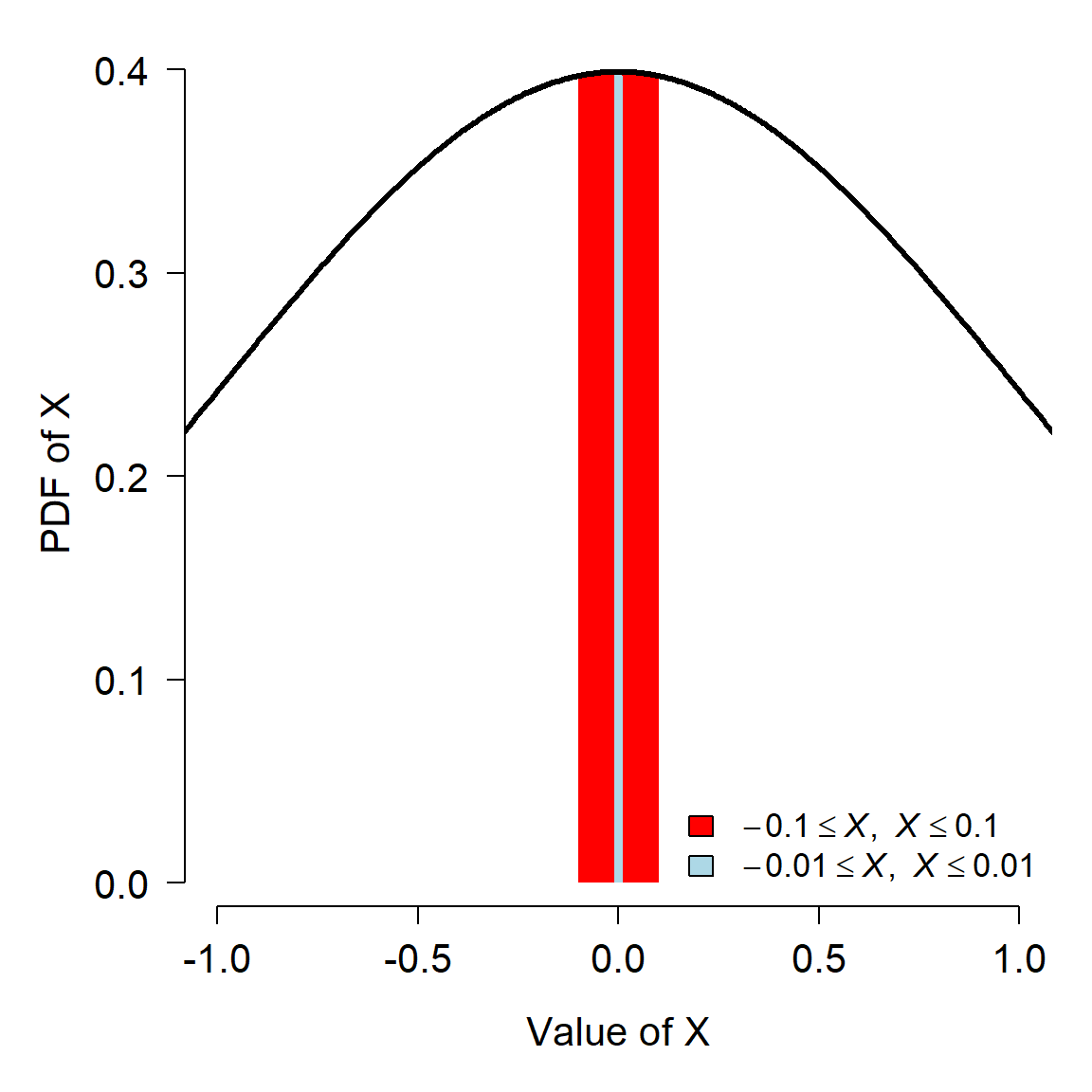
pnorm(0.01)-pnorm(-0.01)[1] 0.007978713Notice that as the interval becomes narrower, its probability becomes smaller. In the limit as the interval shrinks to a single point, the probability becomes 0. This is why the probability of observing any exact value in a continuous distribution is zero, even though the probability of observing values within any finite interval is positive.
Visually, we can see this in the figure below. Notice how the red area is much larger than the light blue area–these are the intervals defined by \(\pm{0.1}\) and \(\pm{0.01}\).
9.3.1 Uniform distribution
The simplest continuous distribution is the uniform distribution. The uniform distribution is parameterized by its upper and lower bounds, usually called \(a\) and \(b\), respectively. All values of a uniform distribution in the interval \(\left[a,b\right]\) are equally likely, and all values outside \(\left[a,b\right]\) have probability 0. The figure below shows the PDFs of 3 different uniform distributions.
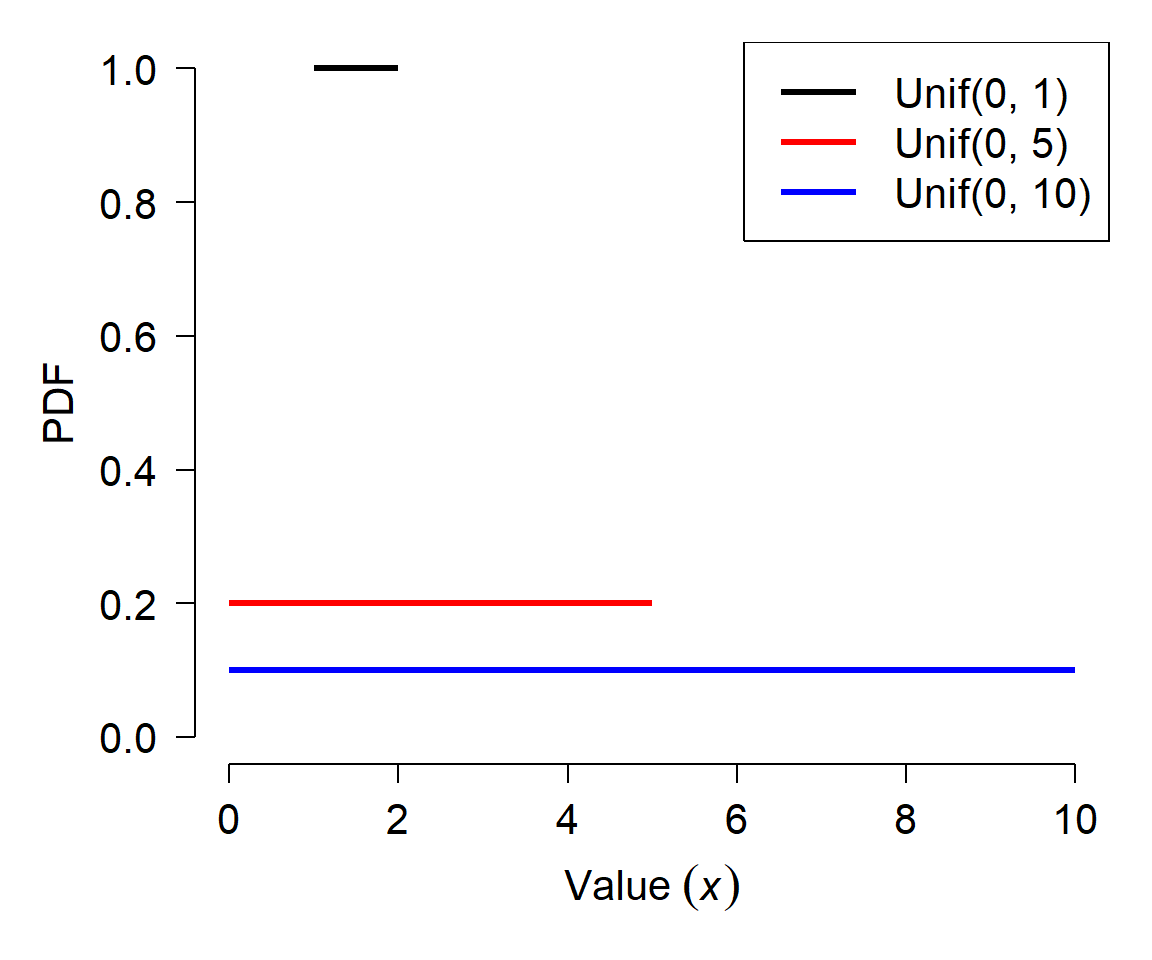
Notice how each distribution has a flat PDF, but that the value of the PDF decreases as the width of the uniform distribution increases. Given what you learned above about the relationship between the CDF and the PDF, can you work out why this is?2
Like the normal distribution, there is a standard uniform distribution that is frequently used. The standard uniform is defined as \(Uniform\left(0,1\right)\): a uniform distribution in the interval \(\left[0,1\right]\). The uniform distribution can sometimes be abbreviated as \(U\left(a,b\right)\) or \(Unif\left(a,b\right)\).
The mean of a uniform distribution is just the mean of its limits:
\[\mu\left(Uniform\left(a,b\right)\right)=\frac{a+b}{2}\]
The variance of a uniform distribution is:
\[\sigma^2\left(Uniform\left(a,b\right)\right)=\frac{{(b-a)}^2}{12}\]
9.3.1.1 Uniform distribution in R
The uniform distribution is accessed using the _unif group of functions, where the space could be d, p, q, or r. These functions calculate or returns something different:
dunif(): Calculates probability density function (PDF) at x.punif(): Calculates CDF, from a up to x. Answers the question, “at what quantile of the distribution should some value fall?”. The reverse ofqunif().qunif(): Calculates the value at a specified quantile or quantiles. The reverse ofpunif().runif(): Draws random numbers from the uniform distribution.
The help files for many R functions include a call to runif() to generate example values from the uniform distribution. This can be confusing to new users, who might interpret “runif” as “run if” (i.e., some sort of conditional statement).
One extremely useful application is the generation of values from the standard uniform distribution:
x <- runif(20)The line above generates 20 numbers from the interval [0, 1]. These values can be used as probabilities or values of a CDF.
If you want to implement a new probability distribution in R, you can use runif() followed by the q__() function that you define for your new distribution to implement a random number generator for it. The example below shows how to implement a “truncated normal” distribution:
rtnorm <- function(N, lower, upper, mu, sigma){
    a <- pnorm(lower, mu, sigma)
    b <- pnorm(upper, mu, sigma)
    x <- runif(N, a, b)
    y <- qnorm(x, mu, sigma)
    return(y)
}

use.n <- 1e3
use.mu <- 10
use.sd <- 3
x1 <- rnorm(use.n, use.mu, use.sd)
x2 <- rtnorm(use.n, 8, 12, use.mu, use.sd)

par(mfrow=c(1,2))
hist(x1, main="Normal", xlim=c(0, 20))
hist(x2, main="Truncated normal", xlim=c(0, 20))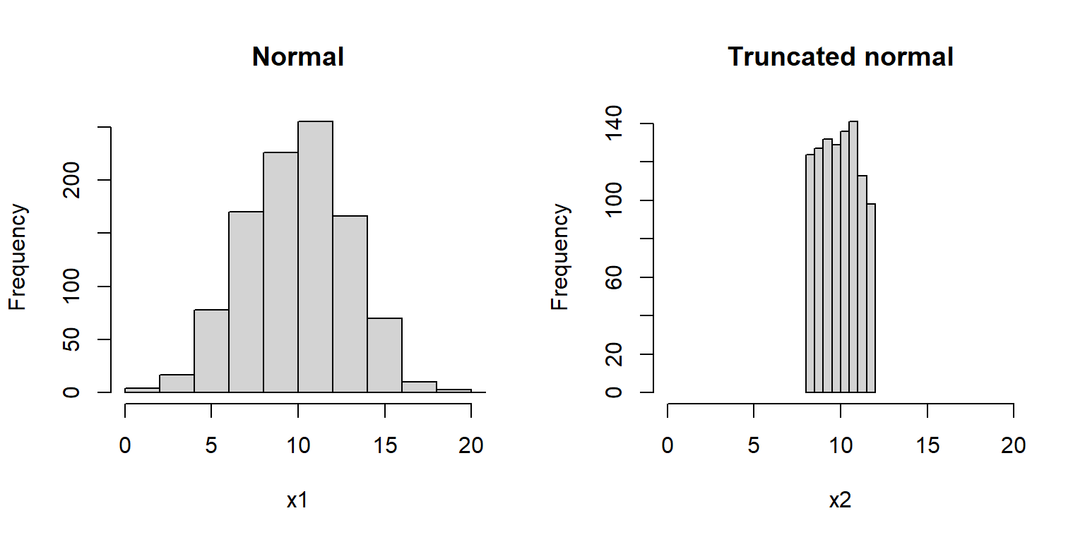
9.3.2 Normal distribution
The normal distribution is probably the most important distribution in statistics. Many natural processes result in normal distributions. Consequently, most classical statistical methods (e.g., t-tests, ANOVA, and linear models) assume that data come from a normal distribution. The normal distribution is also sometimes called the Gaussian distribution because of the work of mathematician Carl Friedrich Gauss, although he did not discover it.
The normal distribution is also sometimes called the bell curve because of the shape of its PDF. This term should be avoided because other probability distributions also have a bell shape, and because normal distributions are not always bell-shaped.
The normal distribution is parameterized by its mean, \(\mu\), and standard deviation, \(\sigma\). Some sources prefer the variance \(\sigma^2\) instead of the standard deviation, and some even use the precision \(1/\sigma^2\) or \(\sigma^{-2}\). This is fine because, as the symbols imply, the SD, variance, and precision are all related. Just pay attention to the notation being used. Using \(\sigma\) instead of \(\sigma^2\) or \(1/\sigma^2\) can be convenient because \(\sigma\) is in the same units as \(\mu\).
The figure below shows several normal distributions with different means and standard deviations.
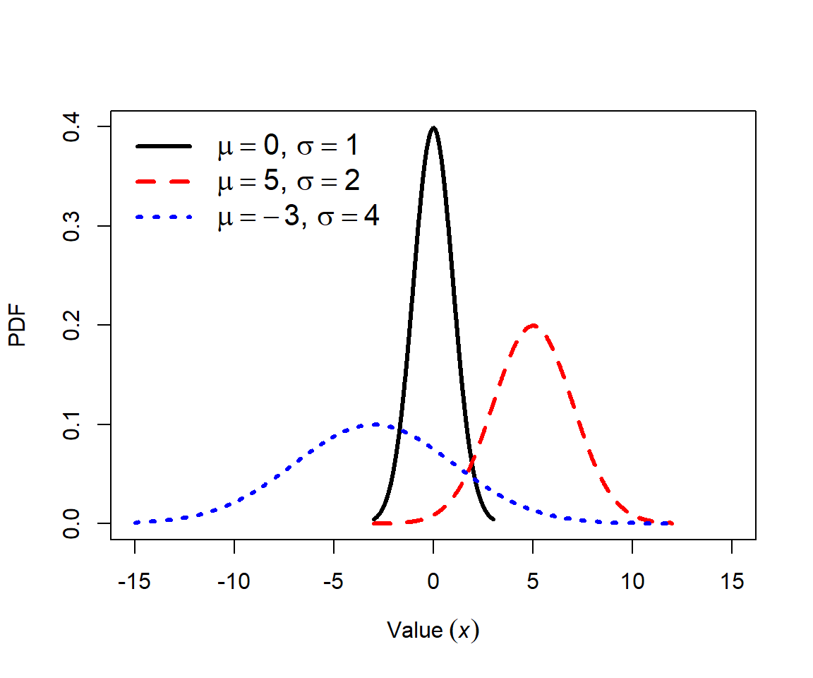
Many phenomena result in normal distributions because of the Central Limit Theorem (CLT). The CLT states that under certain conditions the sum of many random variables will approximate a normal distribution. The main condition is that the random variables will be independent and identically distributed (often abbreviated “i.i.d.”). In other words, the values do not depend on each other, but they all come from the same distribution. The exact distribution does not matter. The example below uses the uniform distribution. The CLT also works with the mean of the random variables instead of the sum, because mean is just the sum scaled by sample size.
# large sample size
N <- 1e4

# set up a vector to hold the sums of
# the random values
xvec <- numeric(N)

# in a loop, draw 10 random values and
# calculate their sum...10000 times
for(i in 1:N){xvec[i] <- sum(runif(10))}

# histogram of the 10000 sums
hist(xvec)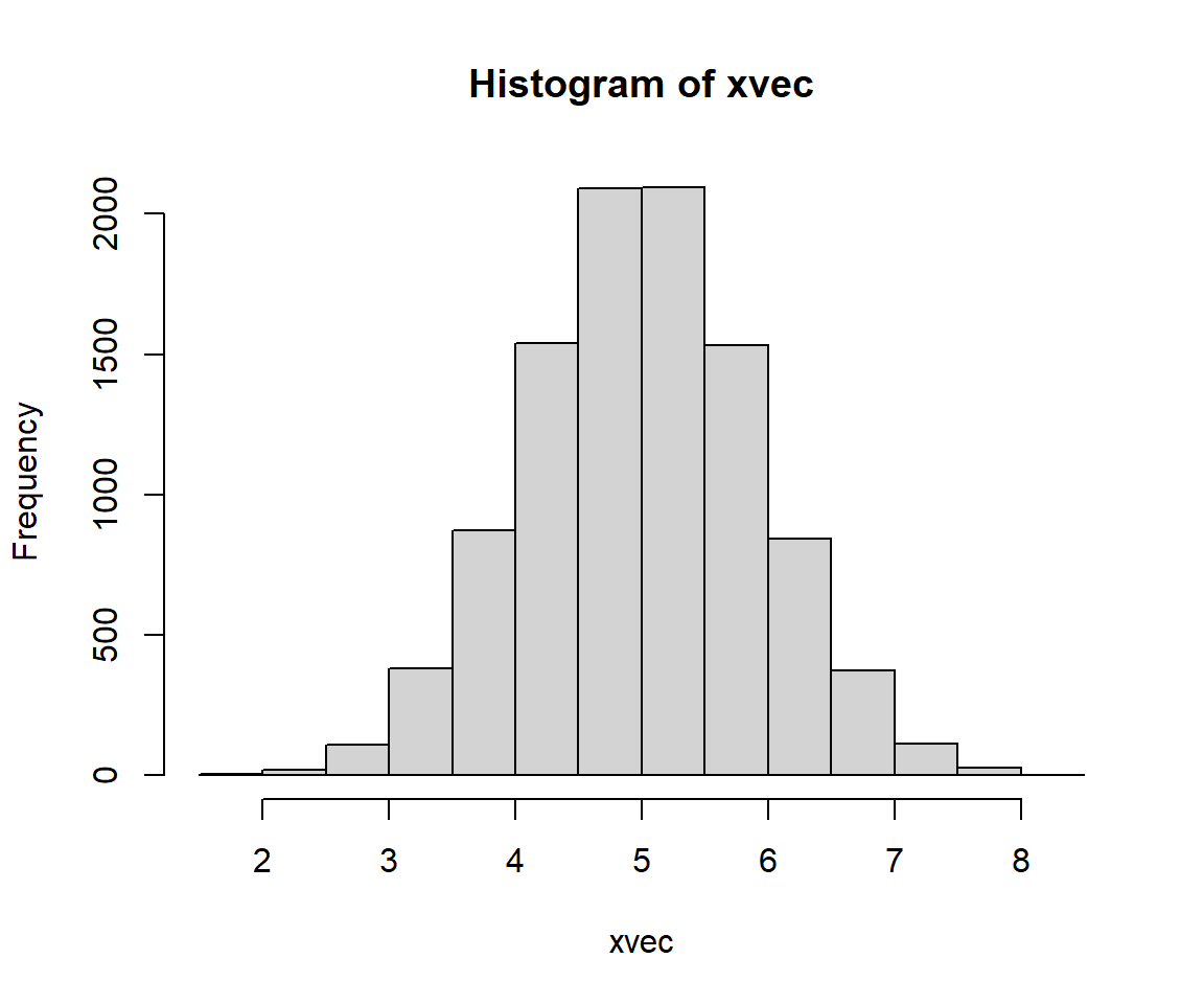
The standard normal distribution has \(\mu=0\) and \(\sigma=1\). This is often written as \(N\left(0,1\right)\). These parameters are the defaults in the R functions that work with the normal distribution.
9.3.2.1 Normal distribution in R
The normal distribution is accessed using the _norm group of functions, where the space could be d, p, q, or r. These functions calculate or returns something different:
dnorm(): Calculates probability density function (PDF) at x.pnorm(): Calculates CDF, from \(-\infty\) up to x. Answers the question, “at what quantile of the distribution should some value fall?”. The reverse ofqnorm().qnorm(): Calculates the value at a specified quantile or quantiles. The reverse ofpnorm().rnorm(): Draws random numbers from the normal distribution.
The normal distribution in R is parameterized by the mean (argument mean) and the SD, not the variance (argument sd). The figure generated below shows the effect of increasing the SD on the shape of a distribution. Greater variance (i.e., greater SD) means that the distribution is more spread out.
mu <- 10
x <- seq(0, 20, by=0.1)
y1 <- dnorm(x, mu, 2)
y2 <- dnorm(x, mu, 5)
y3 <- dnorm(x, mu, 10)

par(mfrow=c(1,1))
plot(x, y1, type="l", lwd=3, xlab="X", ylab="PDF")
points(x, y2, type="l", lwd=3, col="red")
points(x, y3, type="l", lwd=3, col="blue")
legend("topright", legend=c(expression(sigma==2),
        expression(sigma==5), expression(sigma==10)),
        lwd=3, col=c("black", "red", "blue"))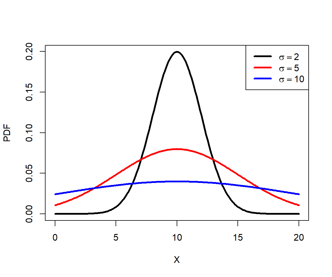
The normal distribution has several useful properties. Generally, the mean and median are the same (if the distribution is not skewed). Approximately 68% of values fall within 1 SD of the mean, 95% of values fall within about 2 SD of the mean (technically 1.9599 SD, or qnorm(0.975)), and 99.7% of values fall within about 3 SD of the mean. So, deviations of \(>3\) SD are very rare and may signify outliers. The number of SD a value falls away from the mean is sometimes referred to as a z-score or a sigma. Z-scores are calculated as:
\[z\left(x\right)=\frac{x-\mu}{\sigma}\]
Where x is the value, \(\mu\) is the mean, and \(\sigma\) is the SD.
Z-scores are sometimes used when comparing variables that are normally distributed, but on very different scales. Converting the raw values to their z-scores is referred to as standardizing them. Any variable, once standardized, has a mean of 0 and SD of 1. The units of a z-scaled variable are “standard deviations away from the mean”.
Standardized values are sometimes used in regression analyses in place of raw values. Many ordination methods such as principal components analysis (PCA) standardize variables automatically. Z-scores (or standardized values) are calculated in R using the scale() function:
x1 <- rnorm(100, 100, 40)
par(mfrow=c(1,2))
hist(x1)
hist(scale(x1))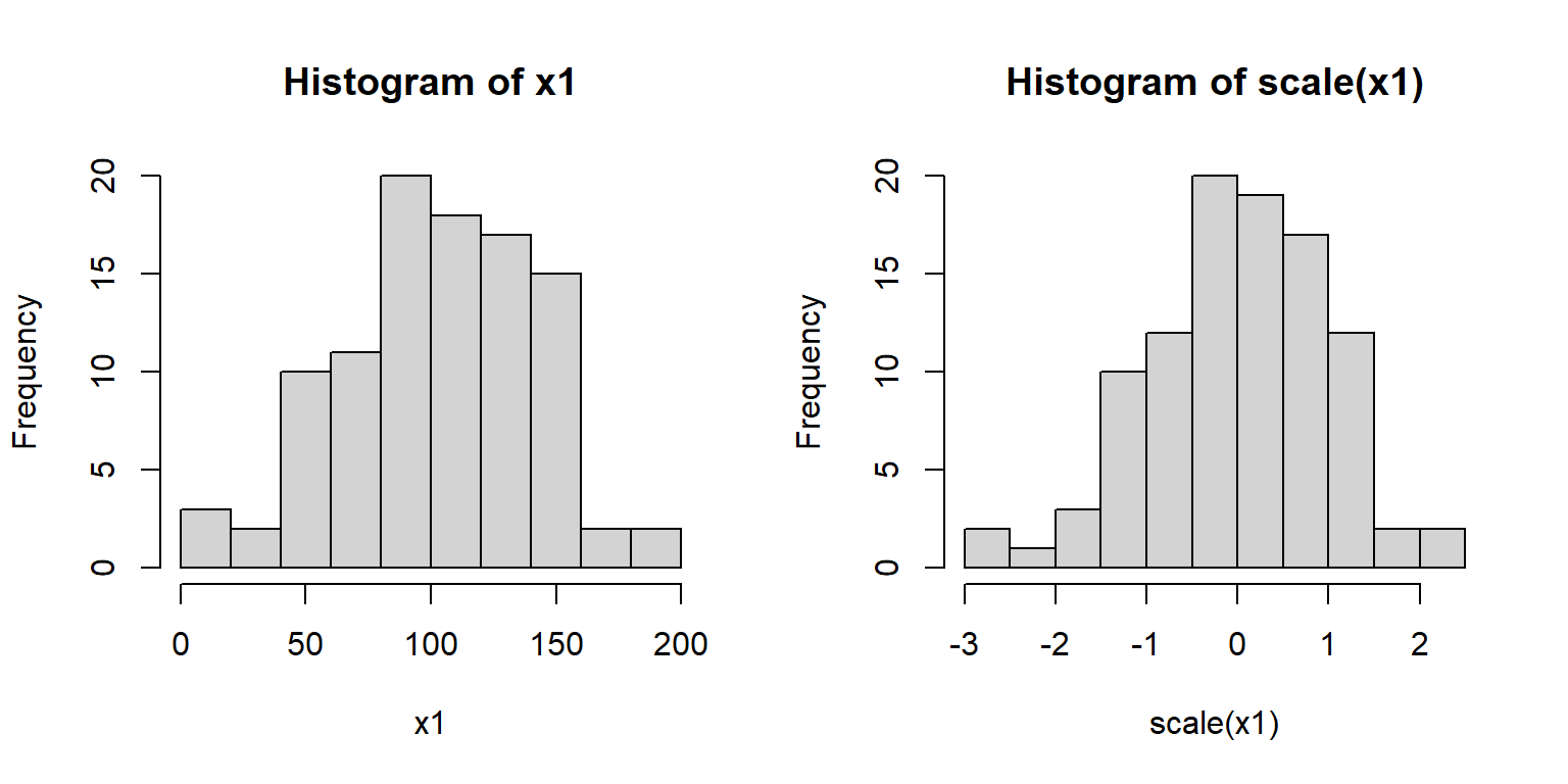
mean(x1)[1] 102.6749sd(x1)[1] 39.16439mean(scale(x1))[1] 1.765851e-16sd(scale(x1))[1] 1Because standardized variables all have the same mean and SD, standardizing a set of variables has the effect of putting all of the variables on equal footing. Without standardizing, variables with larger values or more variance may exert more influence on the analysis than they should simply because of their magnitude.
9.3.3 Lognormal distribution
The lognormal distribution (a.k.a.: log-normal) is, as the name implies, a distribution that is normal on a logarithmic scale. If a variable \(X\) is normally distributed and we exponentiate it, the result \(Z=e^X\) will be lognormally distributed. Conversely, if variable \(Z\) is lognormally distributed, then \(\log\left(Z\right)\) will be normally distributed. By convention the natural log \(\ln\), or \(\log_e\), is used to define the lognormal distribution. R’s lognormal distribution functions use the natural log scale.
The lognormal distribution arises naturally from multiplicative processes. Remember that logarithms relate the operations of multiplication and addition:
\[\log\left(ab\right)=\log\left(a\right)+\log\left(a\right)\]
Suppose some quantity \(z\) is determined by multiplying together many positive numbers:
\[z=X_1X_2X_3\cdots X_n\]
Taking its logarithm gives:
\[\log(Z)=\log(X_1)+\log(X_2)+\log(X_3)+\cdots+\log(X_n)\]
This connects the lognormal distribution to the Central Limit Theorem (Section 9.3.2). The ordinary CLT tells us that the sum of many independent random contributions tends toward a normal distribution under fairly general conditions. If a biological quantity instead results from the product of many independent positive contributions, then taking its logarithm converts that product into a sum. Consequently, the logarithm of the resulting quantity can approach a normal distribution, meaning that the original quantity approaches a lognormal distribution.
This is relevant to many biological processes in which changes are proportional rather than additive. For example, imagine an organism whose size changes during each time interval by a somewhat random growth multiplier. Its final size can be written as
\[S=S_0G_1G_2\cdots G_n\]
where each \(G_i\) is a growth multiplier applied to the starting size \(S_0\). Small random differences in growth therefore accumulate multiplicatively, potentially producing a lognormal distribution of final sizes3.
We can demonstrate the same idea with a simulation. Suppose we repeatedly draw 10 random positive values and multiply them together:
# big sample size (10000)
N <- 1e4
# set up vector for 10000 values
xvec <- numeric(N)
# in a loop, draw 10 random values in [1,2]
# and multiply them all together...10000 times
for(i in 1:N){xvec[i] <- prod(runif(10, 1, 2))}

# plot a histogram of the products,
# and histogram of the log of the products
par(mfrow=c(1,2))
hist(xvec, xlab="Product", main="Original scale")
hist(log(xvec), xlab="Log(Product)", main="Log scale")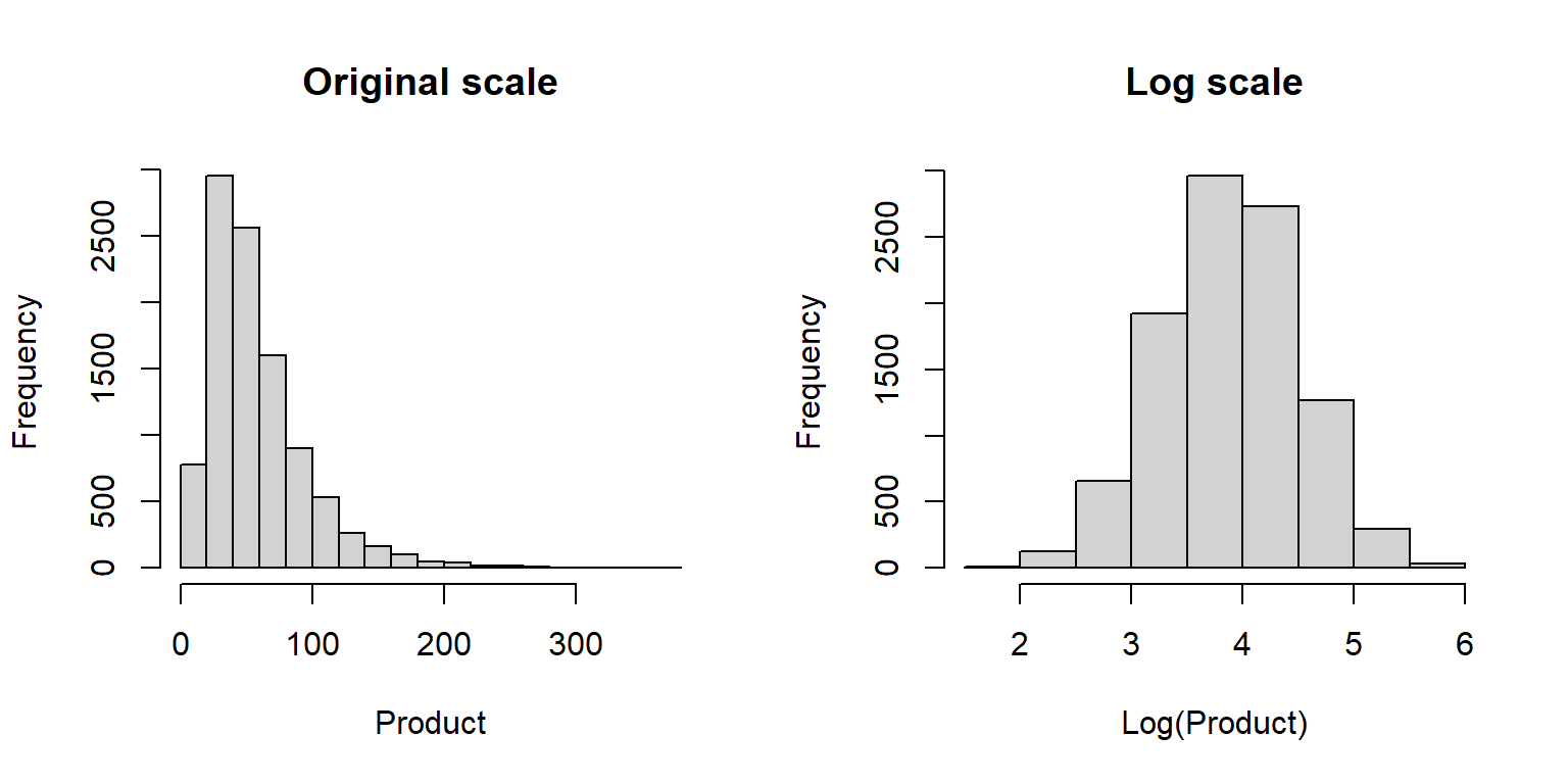
The products in xvec are strongly right skewed on their original scale, but their logarithms are approximately normally distributed. This happens because
\[ \log\left(\prod_{i=1}^{10} X_i\right) = \sum_{i=1}^{10}\log(X_i) \] turning the multiplicative process into an additive one.
More generally, lognormal distributions are useful for describing positive, right-skewed variables in which most observations are relatively small but a few observations are much larger. Such patterns are common in biological measurements including organism sizes, abundances, concentrations, and other quantities influenced by proportional or multiplicative processes. Other positive, right-skewed distributions, particularly the gamma distribution (Section 9.3.4), can produce superficially similar shapes, so the shape of a histogram alone does not establish that a process is lognormal.
The lognormal distribution is parameterized by the mean and standard deviation of the variable after taking its logarithm. In R these parameters are named meanlog and sdlog. Thus, they are not the mean and standard deviation of the lognormally distributed variable on its original scale. Forgetting which quantities are on the log scale is an easy way to produce confusing results, especially when calculating expected values or graphing distributions.
The figure below shows various lognormal distributions with \(\mu=3\) and different SD on a logarithmic scale (left) and a linear scale.
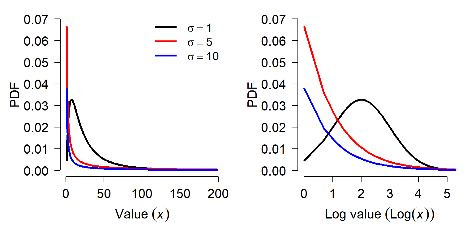
The figures show the effect that variance can have on the lognormal distribution. When the variance on the log scale is \(<\mu\), the distribution is approximately normal on the log scale. As the variance gets larger, the distribution gets more and more right-skewed. Right-skewed means that the values are more and more concentrated near 0, and there are fewer very large values.
Interestingly, the mean of a log-normal distribution is not simply \(e^\mu\) as one might expect. The mean of a lognormal distribution X on the linear scale is
\[mean\left(X\right)=e^{\left(\frac{\mu+\sigma^2}{2}\right)}\]
In this equation, \(\mu\) and \(\sigma\) are the mean and SD on the logarithmic scale, or logmean and logsigma in R terms. The variance on the linear scale is:
\[Var\left(X\right)=e^{2\mu+\sigma^2}\left(e^{\sigma^2}-1\right)\]
What this means is that you cannot transform the parameters of a lognormal distribution from the logarithmic to the linear scale by simply exponentiating or taking logarithms of parameters.
9.3.3.1 Lognormal distribution in R
The lognormal distribution is accessed using the _lnorm group of functions, where the space could be d, p, q, or r. These functions calculate or returns something different:
dlnorm(): Calculates probability density function (PDF) at x.plnorm(): Calculates CDF, from 0 up to x. Answers the question, “at what quantile of the distribution should some value fall?”. The reverse ofqlnorm().qlnorm(): Calculates the value at a specified quantile or quantiles. The reverse ofplnorm().rlnorm(): Draws random numbers from the lognormal distribution.
When working with the lognormal distribution in R it is important to keep in mind that the parameters (meanlog and sdlog) of the _lnorm functions are on the natural log scale. The meanlog parameter is the mean of the logarithm of the values, not the mean of the values or the logarithm of the mean of the values. Similarly, sdlog is the SD of the logarithm of the values, not the SD of the values or the logarithm of the SD of the values. The example below shows this:
# draw some values
x1 <- rlnorm(1e4, 2, 1)

# mean of the values
mean(x1)
[1] 12.16433# mean of the log(values)
mean(log(x1))[1] 1.997859# not the log of the mean of the values
log(mean(x1))[1] 2.498508# sd of the values
sd(x1)[1] 16.08477# sd of the log(values)
sd(log(x1))[1] 0.9971798# exp(meanlog) != mean(x1)
c(exp(2),
mean(x1))[1] 7.389056 12.1643349.3.4 Gamma distribution
The gamma distribution describes waiting times until a certain number of events takes place. This means it is the continuous analogue of the negative binomial distribution, which describes the number of trials until some certain number of successes. The gamma distribution can also be used empirically to describe positive data whose SD is much larger than the mean. This makes it an alternative to the lognormal distribution for right-skewed data, much like the negative binomial is an alternative to the Poisson. Example gamma distributions are shown below.
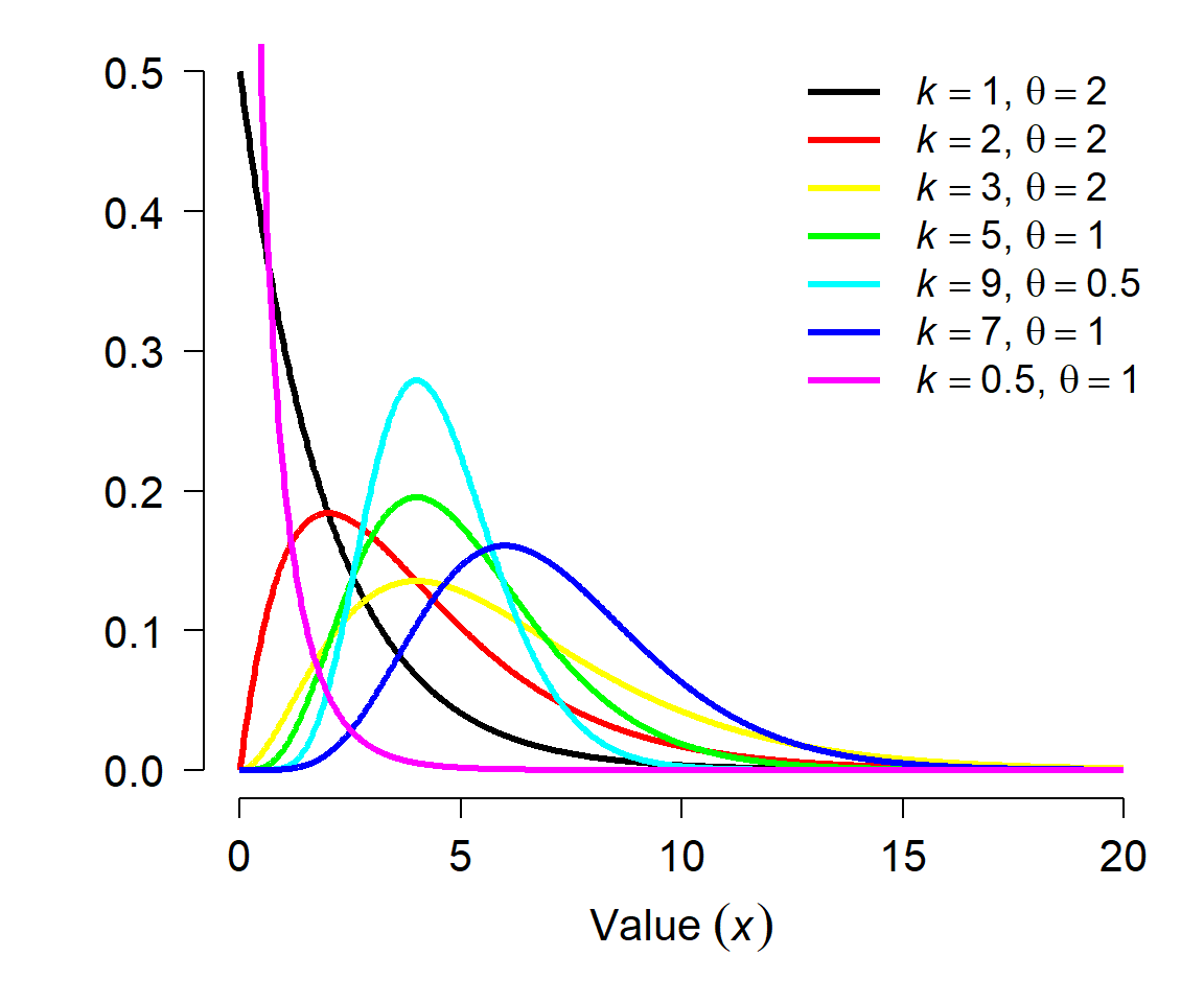
The Gamma distribution is parameterized by its shape and scale.
- The shape parameter \(k\) describes the number of events
- The scale parameter \(\theta\) (“theta”) describes the mean time until each event.
- The scale is sometimes expressed as its reciprocal, the rate.
In R, the gamma can be parameterized by either the shape and scale, or shape and rate. This means you need to name your arguments when working with the gamma distribution.
For example, \(\Gamma(k=4,\theta=2)\) is the distribution of length of time in days it would take to observe 4 events if events occur on average once every two days. Equivalently, it is the time to observe 4 events if events occur at a rate of 1/2 event per day. Consequently, the mean of a gamma distribution given shape \(k\) and scale \(\theta\) (or rate \(r\)) is:
\[\mu=k\theta=\frac{k}{r}\]
The variance is calculated as:
\[\sigma^2=k\theta^2=\frac{k}{r^2}\]
Like the negative binomial, the gamma distribution is often used phenomenologically; that is, used to describe a variable even if its mechanistic description (waiting times) doesn’t make sense biologically. Just as the negative binomial can be used to model count data with variance greater than the mean (i.e., an overdispersed Poisson), a gamma distribution can be used for positive data with \(\sigma\gg\mu\). I.e., the gamma can be used in many of the same cases as the lognormal, although the lognormal may have a clearer biological interpretation.
9.3.4.1 Gamma distribution in R
The gamma distribution is accessed using the _gamma group of functions, where the space could be d, p, q, or r. These functions calculate or returns something different:
dgamma(): Calculates probability density function (PDF) at x.pgamma(): Calculates CDF, from 0 up to x. Answers the question, “at what quantile of the distribution should some value fall?”. The reverse ofqgamma().qgamma(): Calculates the value at a specified quantile or quantiles. The reverse ofpgamma().rgamma(): Draws random numbers from the gamma distribution.
Note that when working with the gamma distribution in R, you must supply either the shape and the rate, or the shape and the scale. Supplying scale and rate will return an error.
# will work:
rgamma(10, shape=3, scale=2)
rgamma(10, shape=3, rate=0.5)

# will return error:
rgamma(10, scale=2, rate=0.5)
9.3.5 Beta distribution
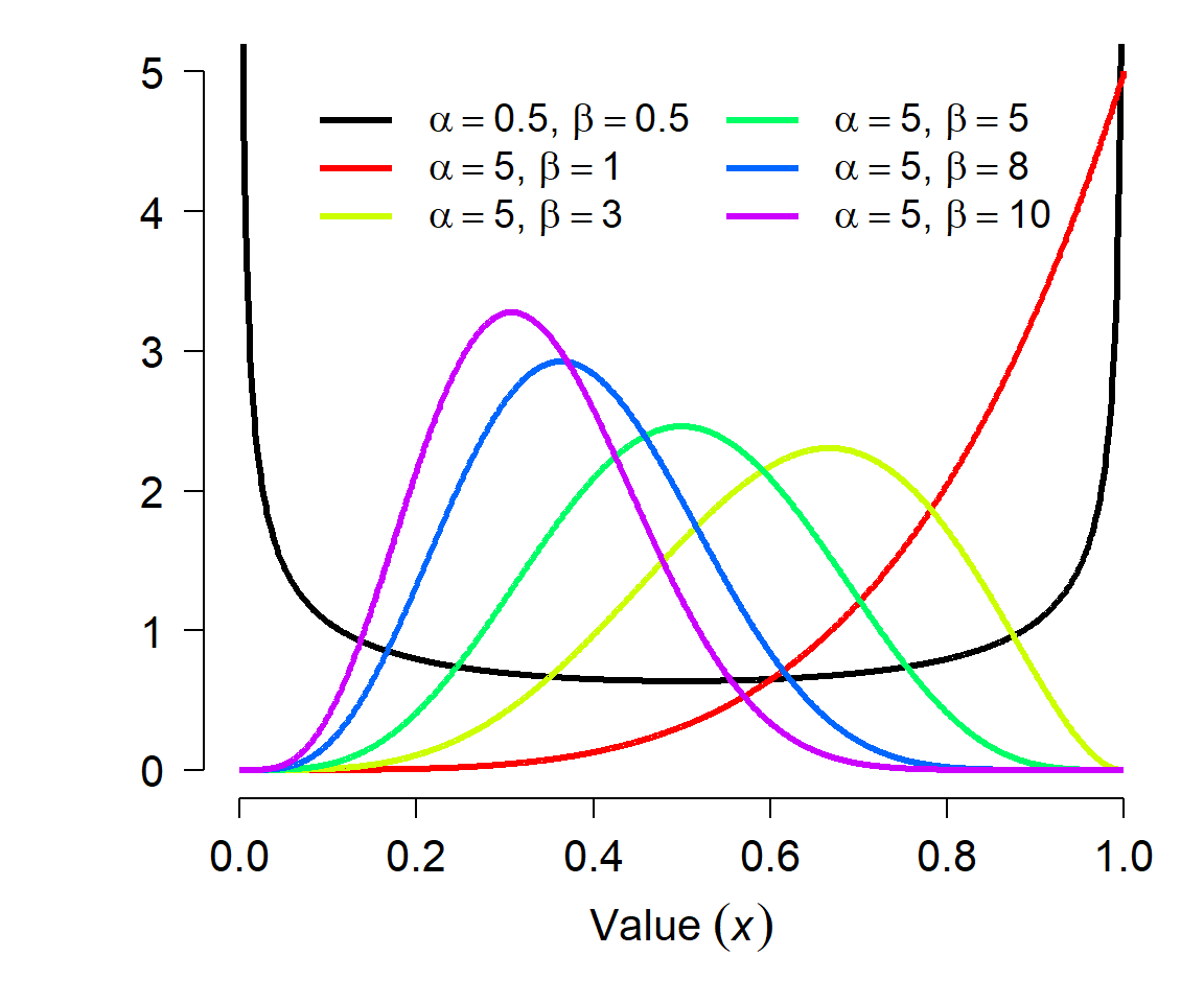
The beta distribution is defined on the interval \([0,1]\) and is parameterized by two positive shape parameters, \(\alpha\) and \(\beta\). For this reason, the beta distribution is often used to model the distribution of probabilities. The beta distribution is probably the most commonly used distribution for variables constrained to lie between 0 and 1, such as probabilities, proportions, and fractions.
The beta distribution is closely related to the binomial distribution. One way to think about the two shape parameters is as summaries of a binomial trial. Parameter \(\alpha\) behaves like the number of successes plus one, while \(\beta\) behaves like the number of failures plus one. This interpretation provides useful intuition for the shape of the distribution: increasing \(\alpha\) shifts probability toward 1, while increasing \(\beta\) shifts probability toward 0. However, \(\alpha\) and \(\beta\) are simply shape parameters and do not have to be integers; but, they do have to be positive.
An even simpler explanation is that the balance of \(\alpha\) and \(\beta\) determine where most of the probability lies. Increasing \(\alpha\) places more probability near 1, whereas increasing \(\beta\) places more probability near 0. Increasing both will crowd the distribution near 0.5. Decreasing both will push the probability out towards 0 and 1 and away from 0.5.
The figure below shows various beta distributions. Notice how probability is shifted toward the center when \(\alpha\) and \(\beta\) both increase, and how the distribution becomes U-shaped when they both decrease.
The beta distribution has mean
\[\mu=\frac{\alpha}{\alpha+\beta}\]
and variance
\[\sigma^2=\frac{\alpha\beta}{\left(\alpha+\beta\right)^2\left(\alpha+\beta+1\right)}\]
These expressions can be re-arranged to solve for \(\alpha\) and \(\beta\) given a mean and variance:
\[\alpha=\left(\frac{1-\mu}{\sigma^2}-\frac{1}{\mu}\right)\mu^2\]
\[\beta=\alpha\left(\frac{1}{\mu}-1\right)\]
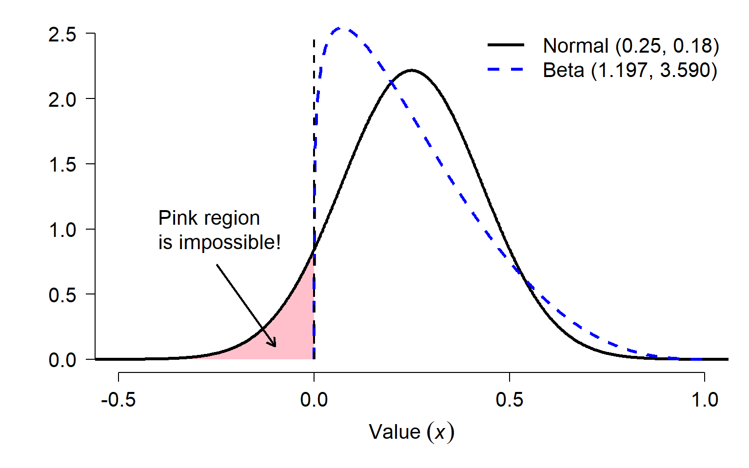
This is useful if you want to use proportions or percentages that were reported as a mean and variance (or SD, or SE). For example, if a paper reports a survival rate estimate as \(0.25\pm0.18\) SE, it’s tempting to misinterpret that as meaning that the survival rate is a normally-distributed variable. However, treating the survival rate as normally distributed would imply that about 8% of the time, the survival rate was negative!
pnorm(0, 0.25, 0.18)[1] 0.08243327So, you should convert these estimates to a beta distribution if you want to understand how they might vary:
\[\alpha=\left(\frac{1-0.25}{\left(0.18\right)^2}-\frac{1}{0.25}\right){0.25}^2\approx1.1968\]
\[\beta=1.1968\left(\frac{1}{0.25}-1\right)\approx3.5903\]
The figure below shows the two distributions, the normal in black and the beta in blue. The dashed vertical line at 0 shows that part of the normal distribution implied by the mean and SE of a survival “probability” is not possible. Converting to a beta distribution preserves the mean and variance while ensuring that all values fall between 0 and 1. This more accurately reflects the true nature of the uncertainty about the probability.
Note that this conversion cannot be done for some combinations of \(\mu\) and \(\sigma\): both \(\alpha\) and \(\beta\) must both be positive, so if you calculate a non-positive value for either parameter then the conversion won’t work. These formulas also require that
\[\sigma^2<\mu\left(1-\mu\right)\]
This can sometimes happen for probabilities very close to 0 or 1 with large variances.
9.3.5.1 Beta distribution in R
The beta distribution is accessed using the _beta group of functions, where the space could be d, p, q, or r. These functions calculate or returns something different:
dbeta(): Calculates probability density function (PDF) at x.pbeta(): Calculates CDF, from 0 up to x. Answers the question, “at what quantile of the distribution should some value fall?”. The reverse ofqbeta().qbeta(): Calculates the value at a specified quantile or quantiles. The reverse ofpbeta().rbeta(): Draws random numbers from the beta distribution.
9.3.5.2 The beta and the binomial
The relationship between the beta and binomial distributions is especially useful for making inferences about probabilities. The binomial distribution describes the number of successes we observe when the probability of success \(p\) is fixed. The beta distribution can instead be used to describe our uncertainty about the value of \(p\) itself.
We can take advantage of the relationship between the binomial and beta distributions to make inferences from count data. Imagine a study where biologists track the probability that fruit flies die before they are 3 weeks old. They report that 30 out of 130 flies die on or before day 21 of life. What can we estimate about the underlying distribution of 3-week survival rates?
One common starting point is to treat all survival probabilities between 0 and 1 as equally plausible before seeing the data. This corresponds to \(\alpha=\beta=1\). We then add the observed successes to \(\alpha\) and failures to \(\beta\).
Then we can model uncertainty either in the survival probability or mortality probability, depending on how we frame successes or failures. If survival is a success, then
\[p_{survival}\sim{Beta\left(\alpha=101,\beta=31\right)}\]
Alternatively, we can model mortality rate using mortality as a success:
\[p_{mortality}\sim{Beta\left(\alpha=31,\beta=101\right)}\]
The mean survival rate is:
Alpha <- 101
Beta <- 31

# mean estimated survival probability
Alpha / (Alpha + Beta)
[1] 0.7651515# middle 95% of distribution
qbeta(c(0.025, 0.975), Alpha, Beta)[1] 0.6894960 0.8332005This tells us that, given our experimental observation of 100 survivors out of 130 flies, that the true underlying survival rate is about 0.765 and is probably in the interval \(\left[0.689,0.833\right]\). We can see that visually below:
# domain of probability
x <- seq(0, 1, length=1e3)

# survival rate distribution
y.surv <- dbeta(x, shape1=101, shape2=31)

par(mfrow=c(1,1), mar=c(5.1, 5.1, 1.1, 1.1),
    bty="n", lend=1, las=1,
    cex.axis=1.3, cex.lab=1.3)
plot(x, y.surv, type="l", lwd=3,
    xlab="P(survival)", ylab="PDF")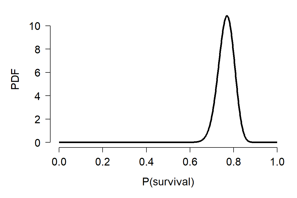
9.3.6 Exponential distribution
The exponential distribution describes the distribution of waiting times until a single event occurs, given a constant rate per unit time of that event occurring. This makes it the continuous analog of the geometric distribution. The exponential distribution is also a special case of the gamma distribution where shape parameter \(k=1\).
The exponential distribution should not be confused with the exponential family of distributions, although the exponential distribution is a member of that family. The exponential family of distributions is a broad class that includes the normal, exponential, gamma, beta, Poisson, and many others.
The exponential distribution is parameterized by a single rate parameter, \(\lambda\), which describes the expected event rate per unit time. For example, \(\lambda=2\) per day means an average waiting time of \(1/0.2=5\) days. It does not mean exactly 0.2 events occur every day–this is a long run average. This property means that \(\lambda\) must be strictly positive. This is exactly the same as the rate parameter r sometimes used to describe the gamma distribution. The mean of an exponential distribution X is:
\[\mu\left(X\right)=\frac{1}{\lambda}\]
and the variance is:
\[\sigma^2\left(X\right)=\frac{1}{\lambda^2}\]
Interestingly, this implies that the standard deviation \(\sigma\) is the same as the mean \(\mu\). Contrast this with the Poisson distribution, where the variance \(\sigma^2\) is the same as the mean. Thus, the CV of the exponential distribution is always 1.
The exponential distribution is supported for all non-negative real numbers; i.e., the half-open interval [0, \(+\infty\)). Like the gamma distribution, the exponential distribution can be used when its mechanistic assumptions make sense, such as waiting times or lifespans with a constant event rate. It also produces strongly right-skewed values, with many small and few large values, but right skew alone is not sufficient reason to assume an exponential distribution.
One other important property of the exponential distribution is that it is memoryless. If the event rate is constant, then the probability of waiting an additional amount of time does not depend on how long you have already waited. For example, if mortality follows an exponential distribution with a constant hazard, an individual that has already survived 5 years has the same expected remaining lifespan as a newly observed individual. The memoryless property is related to why the gambler’s fallacy is a fallacy. If independent events occur with constant probability or rate, a long period without an event does not make that event “due.” The geometric distribution has this property in discrete time, and the exponential distribution has the analogous property in continuous time.
9.3.6.1 Exponential distribution in R
The exponential distribution is accessed using the _exp group of functions, where the space could be d, p, q, or r. These functions calculate or returns something different:
dexp(): Calculates probability density function (PDF) at \(x\).pexp(): Calculates the cumulative probability \(P\left(X\leq{x}\right)\). I.e., it tell you what proportion of the distribution lies at or below a specified value. The reverse ofqexp().qexp(): Calculates the value at a specified quantile or quantiles. The reverse ofpexp().rexp(): Draws random numbers from the exponential distribution.
9.3.7 Triangular distribution
The triangular distribution is sometimes used as a simple “lack of knowledge” distribution when little information is available beyond a plausible minimum, maximum, and most likely value. It is used more often to represent uncertainty in simulations and risk models than to model observed biological data directly.
Sometimes we need to model a process about which we have very little information. For example, we may want to simulate population dynamics without knowing a key survival rate, or organismal growth without knowing a key growth constant. In these situations we might have only a vague idea of how a parameter or an outcome are distributed. At a minimum, we can usually infer or estimate the range and central tendency of a variable. Those are enough to estimate a triangular distribution.
The triangular distribution has three parameters: the lower limit \(a\), the upper limit \(b\), and the mode (most common value) \(c\). Any triangular distribution must satisfy \(a<b\) and \(a\le{c}\le{b}\).
The mean of a triangular distribution X is the mean of its parameters:
\[\mu\left(X\right)=\frac{a+b+c}{3}\]
and the variance is
\[\sigma^2\left(X\right)=\frac{a^2+b^2+c^2-ab-ac-bc}{18}\]
In addition to serving as a stand-in distribution when data are scarce, the triangular distribution can arise in several natural situations. For example, the mean of two standard uniform variables follows a triangular distribution (see below).
9.3.7.1 Triangular distribution in R
The triangular distribution is available in the add-on package extraDistr (Wolodzko 2026). The triangular distribution is accessed using the _triang group of functions, where the space could be d, p, q, or r. These functions calculate or returns something different:
dtriang(): Calculates probability density function (PDF) at \(x\).ptriang(): Calculates \(P\left(X\le{x}\right)\), the CDF from \(a\) to \(x\). The reverse ofqtriang().qtriang(): Calculates the value at a specified quantile or quantiles. The reverse ofptriang().rtriang(): Draws random numbers from the triangular distribution.
The code below shows the PDFs of various triangular distributions. Notice that c is not used as a variable name, to avoid potentially masking the very critical R function c.
library(extraDistr)
ax <- c(1,1,3)
bx <- c(5, 10, 7)
cx <- c(3, 3, 6)

x1 <- seq(ax[1], bx[1], length=50)
x2 <- seq(ax[2], bx[2], length=50)
x3 <- seq(ax[3], bx[3], length=50)
y1 <- dtriang(x1, ax[1], bx[1], cx[1])
y2 <- dtriang(x2, ax[2], bx[2], cx[2])
y3 <- dtriang(x3, ax[3], bx[3], cx[3])

plot(x1, y1, type="l", lwd=3, xlab="X", ylab="PDF",
     xlim=c(0, 10))
points(x2, y2, type="l", lwd=3, col="red")
points(x3, y3, type="l", lwd=3, col="blue")
legend("topright", legend=c("Tri(1, 5, 3)", "Tri(1, 10, 3)", "Tri(3, 7, 6)"),
       lwd=3, col=c("black", "red", "blue"))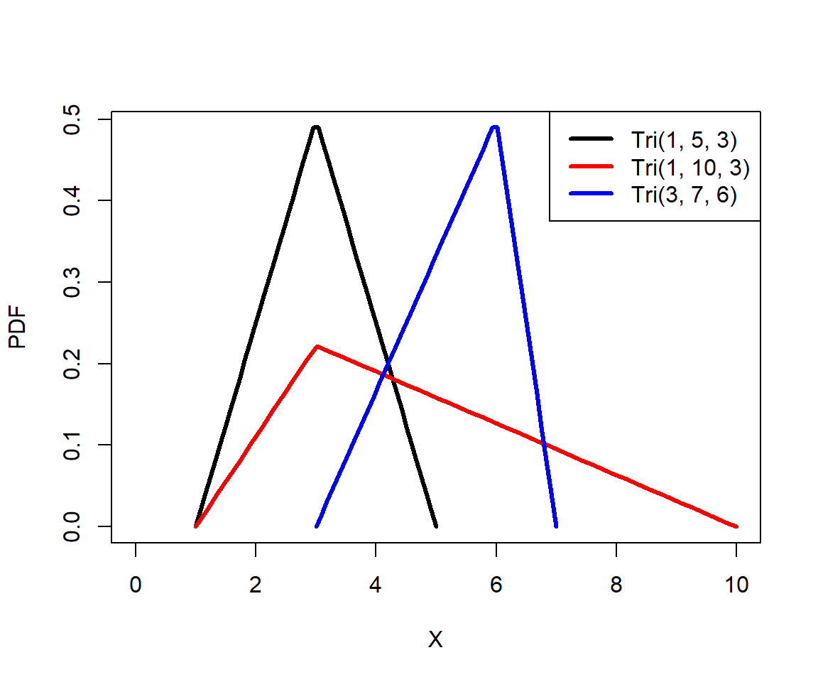
The code below demonstrates how a triangular distribution can arise as the distribution of means of two standard uniform variables x1 and x2. The command density() calculates the kernel density estimate of a vector. This kernel density estimate is an empirical estimate of the PDF of a variable.
# random number seed for reproducibility
set.seed(42)

# sample size
n <- 10^(2:4)

# set up lists to hold simulation results
x1 <- vector("list", length(n))
y <- vector("list", length(n))
x <- vector("list", length(n))

# simulate uniforms in a for loop
for(i in 1:length(n)){
    x[[i]] <- (runif(n[i]) + runif(n[i]))/2
}

# calculate the empirical density function
for(i in 1:length(n)){
    z <- density(x[[i]])
    x1[[i]] <- z$x
    y[[i]] <- z$y
}

# make the graph
cols <- rainbow(3)
plot(x1[[1]], y[[1]], type="l", lwd=3, col=cols[1],
     xlab="X", ylab="Kernel density estimate", ylim=c(0, 2))
for(i in 2:3){
    points(x1[[i]], y[[i]], type="l", lwd=3, col=cols[i])
}
legend("topleft", legend=c("n=100", "n=1000", "n=10000", "triangular"),
    bty="n", lwd=3, col=c(cols[1:3],"black"), lty=c(1,1,1,2))
# add the triangular distribution
curve(dtriang(x, 0, 1, 0.5), from=0, to=1, add=TRUE, lwd=3, lty=2)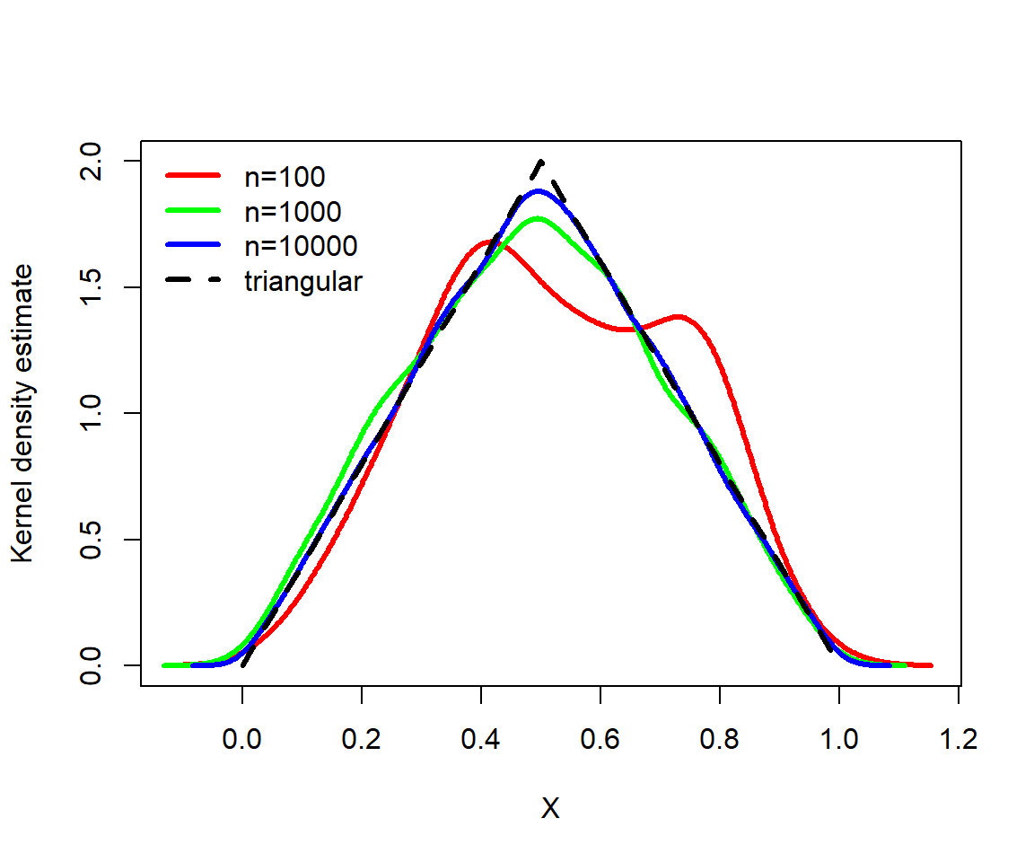
9.3.8 Distribution summary
The table below summarizes some the key features of the discrete distributions we explored in this module.
| Distribution | Support | What it models |
|---|---|---|
| Bernoulli | \(x\in\{0,1\}\) | Outcome of a single binary trial |
| Binomial | \(x\in\{0,1,\ldots,n\}\) | Number of successes in \(n\) independent trials with constant probability \(p\) |
| Poisson | \(x\in\{0,1,2,\ldots\}\) | Number of events occurring independently at a constant rate |
| Negative binomial | \(x\in\{0,1,2,\ldots\}\) | Number of failures before a specified number of successes; commonly used for overdispersed count data |
| Geometric | \(x\in\{0,1,2,\ldots\}\) | Number of failures before the first success, with constant probability \(p\) |
| Beta-binomial | \(x\in\{0,1,\ldots,n\}\) | Number of successes in \(n\) trials when the probability \(p\) varies |
| Multinomial | \(x_i\in\{0,1,\ldots,n\}\), with \(\sum_i x_i=n\) | Counts among \(k\) categories from \(n\) trials |
The table below summarizes some the key features of the continuous distributions we explored in this module.
| Distribution | Support | What it models |
|---|---|---|
| Uniform | \(x\in[a,b]\) | Continuous variables where all values within a bounded interval are equally likely |
| Normal | \(x\in(-\infty,+\infty)\) | Continuous variables arising from many additive processes; symmetric data concentrated around a mean |
| Lognormal | \(x\in(0,+\infty)\) | Positive variables that are normally distributed on a log scale; often arise from multiplicative processes |
| Gamma | \(x\in(0,+\infty)\) | Positive, right-skewed variables; waiting times until a specified number of events occurring at a constant rate |
| Beta | \(x\in[0,1]\) | Continuous proportions and probabilities, including uncertainty about the probability of a binary event |
| Exponential | \(x\in[0,+\infty)\) | Waiting times until the first event when events occur at a constant rate |
| Triangular | \(x\in[a,b]\) | Bounded continuous variables when only the minimum, maximum, and most likely value are known |
Wolodzko T. 2026. extraDistr: Additional univariate and multivariate distributions.
Although the values must be rounded to non-negative integers!↩︎
The area under the PDF must be 1, so the height of the PDF of a uniform distribution must be 1 divided by its width.↩︎
If the growth factors \(G_n\) are constant, then \(S_t=S_0G^t\), or more generally an exponential function \(f\left(t\right)=ae^{bt}\). Attempting to calculate the derivative of this function leads to preferring Euler’s constant \(e\) as the base because the function \(e^t\) is it’s own derivative. Here is a youtube video that explains this visually.↩︎