# make a matrix from the table above
a <- matrix(c(17,6,3,4,4,14), byrow=TRUE, nrow=3)
a
[,1] [,2]
[1,] 17 6
[2,] 3 4
[3,] 4 14Tests for contingency, or tests for independence, are tests where both the predictor and the response variables are categorical. The question being asked is usually some version of, “If an observation is in category A, does it also tend to be in category B?”.
Consider the (made up) data from a pesticide exposure experiment below:
| Pollen production | Unexposed | Exposed |
|---|---|---|
| None | 17 | 6 |
| Reduced | 3 | 4 |
| Normal | 4 | 14 |
This table tallies the fates of 48 plants that were exposed or not exposed to an experimental pesticide. The outcomes were classified as no pollen production, reduced pollen production, and normal pollen production. Rather than asking a question about the mean pollen production in each group, the researchers might ask whether the fate of a plant (in terms of pollen production) is independent of whether or not it was treated. This is why the tests in this module are sometimes called tests of independence.
A good clue for whether or not you need to do a test for independence is whether or not your data are best summarized in a contingency table (Section 7.3.2). A contingency table shows how often observations fall into each category within a dataset.
Fisher’s exact test is a test for independence in contingency tables that is usually only used when expected values are small (\(\lessapprox5\)) or when the \(\chi^2\) test gives questionable approximations.
Question: Are the proportions of data described by two or more categorical variables random or nonrandom?
Null hypothesis: Membership in one of one set of categories is independent of membership in one of another set of categories.
Alternative hypothesis: Membership in one of one set of categories is not independent of membership in one of another set of categories.
Example use case: Rick is studying if whether a fish spawning or not spawning is related to whether it resides in main channel or off-channel habitat, and he has dozens of fish in his dataset.
Fisher’s exact test is a test for independence in contingency tables that is usually only used when the some of the expected values are 5 or less. Although historically it was not used at large sample sizes because the p-value calculation involves numerous factorials that were intractable with older computers, modern algorithms can use computational shortcuts to shorten this substantially. In fact, the Fisher’s exact test is valid at any sample size, but tends to be more conservative than alternatives like the \(\chi^2\) test.
# make a matrix from the table above
a <- matrix(c(17,6,3,4,4,14), byrow=TRUE, nrow=3)
a [,1] [,2]
[1,] 17 6
[2,] 3 4
[3,] 4 14The expected values, ironically, can be calculated by the chisq.test() function:
chisq.test(a)$expected [,1] [,2]
[1,] 11.5 11.5
[2,] 3.5 3.5
[3,] 9.0 9.0Notice that some of the expected cell counts are less than 5. In such situations, the \(\chi^2\) approximation can be suspect and the Fisher’s test is preferred.
fisher.test(a)
    Fisher's Exact Test for Count Data

data:  a
p-value = 0.002849
alternative hypothesis: two.sided
Because Fisher’s is an exact test (i.e., the P-value is an direct, exact calculation), there are no test statistics or degrees of freedom to report.
The chi-square (\(\chi^2\)) test is a more powerful, flexible, and computationally efficient cousin of the Fisher’s exact test. It works by comparing the input contingency table to what the contingency table would be expected to look like under the assumption of independence. That is, if the null hypothesis were true. The test statistic, \(\chi^2\), measures how different the two contingency tables are. The test works better with large sample sizes; with small sample sizes, the approximations use to estimate the p-value can break down. A good rule of thumb is that every cell (or most cells) of the hypothetical null contingency table should have \(\geq5\) observations.
To meet the \(E\left(n\right)\ge5\) criterion, we need to collect more data for our imaginary pesticide experiment above. Consider the (made up) data from a pesticide exposure experiment below:
| Pollen production | Unexposed | Exposed |
|---|---|---|
| None | 33 | 15 |
| Reduced | 8 | 13 |
| Normal | 9 | 22 |
# make a matrix from the table above
b <- matrix(c(33, 15, 8, 13, 9, 22), byrow=TRUE, nrow=3)
b
[,1] [,2]
[1,] 33 15
[2,] 8 13
[3,] 9 22The \(\chi^2\) test assumes that every outcome category is equally likely within every input category. In other words, input and outcome categories are independent of each other. The expected cell counts can be calculated by scaling observed cell counts by the marginal and grand total:
| Pollen production | Unexposed | Exposed | Row totals |
|---|---|---|---|
| None | 33 | 15 | 48 |
| Reduced | 8 | 13 | 21 |
| Normal | 9 | 22 | 31 |
| Column totals | 50 | 50 | 100 |
The expected count in the cell in row \(i\), column \(j\), is:
\[E_{ij}=\frac{R_iC_j}{T}\]
where \(R_i\) is the total for row \(i\), \(C_j\) is the total for column \(j\), and \(T\) is the grand total. For example, for row 1, column 2, the expected value is:
\[E_{1,2}=\frac{48\cdot50}{100}=24\]
So the entire table is:
| Pollen production | Unexposed | Exposed | Row totals |
|---|---|---|---|
| None | \(\left(48\cdot50\right)/100=24\) | \(\left(48\cdot50\right)/100=24\) | 48 |
| Reduced | \(\left(21\cdot50\right)/100=10.5\) | \(\left(21\cdot50\right)/100=10.5\) | 21 |
| Normal | \(\left(31\cdot50\right)/100=15.5\) | \(\left(31\cdot50\right)/100=15.5\) | 31 |
| Column totals | 50 | 50 | 100 |
Once we have the expected counts, we can calculate the \(\chi^2\) statistic as:
\[\chi_{stat}^2=\sum_{i=1}^{n_{row}}\sum_{j=1}^{n_{col}}\frac{\left(O_{ij}-E_{ij}\right)^2}{E_{ij}}\]
The \(\chi^2\) statistic is then compared to a \(\chi^2\) distribution with \(\left(n_{row}-1\right)\left(n_{col}-1\right)\) degrees of freedom. In this case, \(DF=\left(3-1\right)\left(2-1\right)=2\). The p-value is then calculated as:
1-pchisq(13.392, 2)[1] 0.001235845Fortunately, we don’t have to calculate all of that by hand. The chisq() function includes the expected counts in its output object, and prints everything you need to report in your write-up. The \(\chi^2\) test is not an exact test, so you need to report the test statistic and degrees of freedom.
# chi squared test
chi.b <- chisq.test(b)
chi.b
    Pearson's Chi-squared test

data:  b
X-squared = 13.392, df = 2, p-value = 0.001236
In your manuscript, thesis, or whatever, the test would be reported as, “pollen production class was not independent of pesticide application (\(\chi^2=13.39\), 2 d.f., p = 0.001)”.
Let’s check the expected counts to make sure none are \(<5\).
# check the expected counts
# if >1 are <5, consider a Fisher's exact test
chi.b$expected
[,1] [,2]
[1,] 24.0 24.0
[2,] 10.5 10.5
[3,] 15.5 15.5The G-test is another test for independence that can be used in situations where the \(\chi^2\) test is appropriate. It’s main advantage is that it is more computationally efficient at very large sample sizes (1000s or more). Its test statistic is a bit different:
\[ G=2\sum_{i}^{n}{O_ilog{\left(\frac{O_i}{E_i}\right)}} \]
Where the terms are the same as in the equation for \(\chi^2\) and “log” is the natural logarithm function. Further, the total observed count must equal the total expected count:
\[ \sum_{i}^{n} O_i=\sum_{i}^{n} E_i \]
The G-test should be used when sample sizes are large, because it is more computationally efficient than \(\chi^2\), and in situations where \(O_i>2E_i\) for at least some cells.
Despite that fact that is has been recommended in literature for over 3 decades, the G-test is not available in the base R stats package. It is implemented in several add-on packages such as AMR.
McNemar’s test is essentially the paired-data counterpart of a chi-squared test for two samples for two binary variables. Sometimes we collect data on a categorical outcome from the same experimental units at two occasions, with the idea being to compare the change from one time to another–say, before and after some intervention. For example, imagine you are studying the prevalence of some nematode parasite in a population of 100 mice. You test each mouse for infection, administer an antihelminthic, and test the same mice again 3 weeks later. The data might look like this:
| After: Infected | After: Not infected | Row totals | |
|---|---|---|---|
| Before: Infected | 20 | 30 | 50 |
| Before: Not infected | 10 | 40 | 50 |
| Column totals | 30 | 70 | 100 |
And you might think of trying a chi-squared test. But, an ordinary Pearson chi-squared test would be inappropriate because each mouse contributes not one, but two observations. So, a chi-squared test asks the question, “Is the probability of a mouse being in the”After: Not infected” group or the “After: Infected group” independent of whether that mouse was in the “Before: Not infected” or “Before: Infected” group?“. McNemar’s test asks,”Is the probability of changing from infected to uninfected equal to the probability of changing from uninfected to infected?”
McNemar’s test works by considering only the discordant pairs. For the data above, we have:
The 60 mice that didn’t change status don’t tell us much about the direction of change. Consequently, they don’t contribute to the test statistic. For a \(2\times2\) table, we define:
Then calculate the McNemar version of the \(\chi^2\) statistic:
\[\chi^2_{McNemar}=\frac{\left(b-c\right)^2}{b+c}\]
In the example,
\[\chi^2_{McNemar}=\frac{\left(30-10\right)^2}{30+10}=10\]
This statistic follows a \(\chi^2\) distribution with one degree of freedom, giving us \(p\approx0.0016\). This test is deceptively simple: if 40 mice changed status, how unlikely was it that 30 of those 40 were in one direction?
If that last question reminds you of a binomial question, then you are paying attention. That version of that question is the same as asking, “If we flip 40 fair coins, did we get a highly unlikely number of heads or tails?” We can estimate the probability of getting 10 or fewer heads, or 30 or more heads, like this:
sum(dbinom(c(0:10, 30:40), 40, 0.5))[1] 0.002221434Or visually:
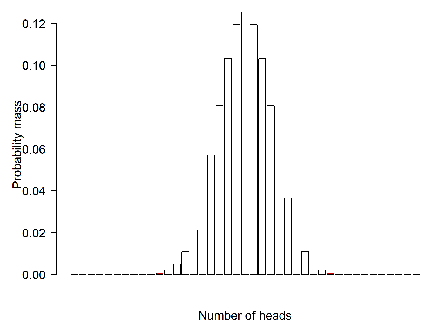
The exact McNemar test is just a binomial sign test applied to the discordant pairs. Under the null hypothesis that \(p\left(Infected\rightarrow~Uninfected\right)=p\left(Uninfected\rightarrow~Infected\right)\),
\[b\sim~Binomial\left(n=b+c,p=0.5\right)\]
So in R we can perform:
binom.test(30, 40, p=0.5)
    Exact binomial test

data:  30 and 40
number of successes = 30, number of trials = 40, p-value = 0.002221
alternative hypothesis: true probability of success is not equal to 0.5
95 percent confidence interval:
 0.5880380 0.8730852
sample estimates:
probability of success
                  0.75
The \(p\)-value may differ a bit from the actual McNemar test because the latter uses a chi-square approximation.
R has a built-in fuction, mcnemar.test(), which accepts a \(2\times2\) contingency table:
a <- matrix(c(20, 10, 30, 40), nrow=2)
mcnemar.test(a)
    McNemar's Chi-squared test with continuity correction

data:  a
McNemar's chi-squared = 9.025, df = 1, p-value = 0.002663
By default, R applies a small correction (“continuity correction”) which makes the test more conservative.
\[\chi^2_{McNemar}=\frac{\left(\left|b-c\right|-1\right)^2}{b+c}\]
There are also extensions of McNemar’s test for more than two categories, often called the McNemar–Bowker test or Bowker’s test of symmetry.
One interesting way to express the results of a test for independence is to use the odds ratio of one outcome relative to another. The odds of some event \(k\) with probability \(p\) is:
\[Odds\left(k\right)=\frac{p\left(k\right)}{1-p\left(k\right)}\]
So the odds ratio of two events \(k\) and \(m\) is simply the odds of \(k\) divided by the odds of \(\neg k\).
\[OR\left(k,m\right)=\frac{\frac{p\left(k\right)}{1-p\left(k\right)}}{\frac{p\left(m\right)}{1-p\left(m\right)}}\]
Odds ratios make it easier to interpret relative likelihoods than probabilities. For example, if the control treatment in some experiment results in 96% mortality, and the other treatment has 98% mortality, the effect size of the treatment is not 2%. It is really \(\left(\left(0.98\right)/\left(0.02\right)\right)/\left(\left(0.96\right)/\left(0.04\right)\right)=2.04\). That is, the treatment more than doubled the likelihood of mortality! Expressing that result as an odds ratio feels like it is overstating things, until you realize that the proportion of non-mortalities was cut in half. If the mortality rates were lower, say 52% vs. 54%, the odds ratio would be 1.08, meaning that mortality was 8% more likely than in the control.
Let’s calculate the odds ratios for our pesticide study. Collapse the 3 outcomes into 2: normal pollen, and less than normal pollen (which includes no pollen):
| Pollen production | Unexposed | Exposed | Row totals |
|---|---|---|---|
| Reduced | 41 | 28 | 69 |
| Normal | 9 | 22 | 31 |
| Column totals | 50 | 50 | 100 |
The odds ratio for reduced pollen in the exposed treatment compared to control is:
\[\frac{\frac{28}{22}}{\frac{41}{8}}=\frac{1.273}{4.556}=0.248\]
This means that plants in the exposed treatment were 0.248 times as likely to have reduced pollen production as plants in the control treatment. Or, you could reverse the calculation and find that exposed plants were 4.03 times as likely to have normal pollen counts.