22  Nonlinear methods for biology

Many biological processes and phenomena are related in ways that do not form straight lines. What this really means is that rates of change are not constant. While linear models and the assumption of linearity are powerful ways to think about and analyze biological phenomena, they are not always appropriate. This module will introduce you to some ways of exploring situations where one quantity does not scale as a constant proportion of another.

So far we have learned about a wide variety of linear models, generalized and otherwise. Linear models predict some response variable \(y\) as a linear function of one or more predictor variables \(x\). One key feature of linear functions is that their slopes are constant. Each model coefficient describes the change in \(Y\) per unit change in \(X\). As we saw in Section 16.2.1, many functions that appear nonlinear at first can be made linear by transforming one or both of \(Y\) and \(X\).

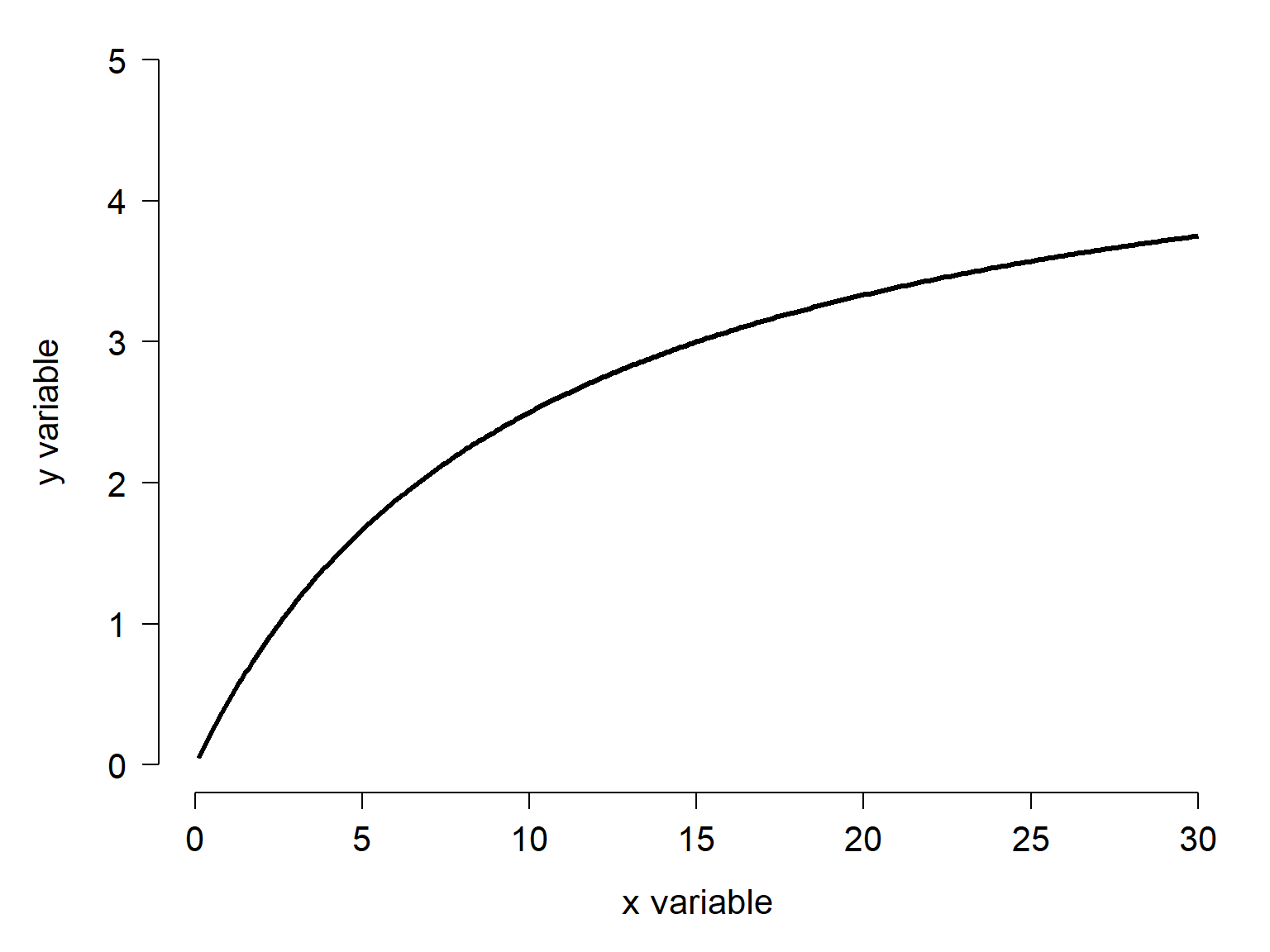
But some functions cannot be transformed to linearity. Consider the function below.

Figure 22.1: The Michaelis-Menten function is a famous nonlinear function that cannot be transformed to linearity.

At first glance, this looks like a power law with an exponent between 0 and 1. If that were the case, we could linearize it by log-transforming \(x\) and \(y\). But, it turns out that the function is not linear under those conditions:

Figure 22.2: Even if you log-transform both x and y, the Michaelis-Menten function remains nonlinear.

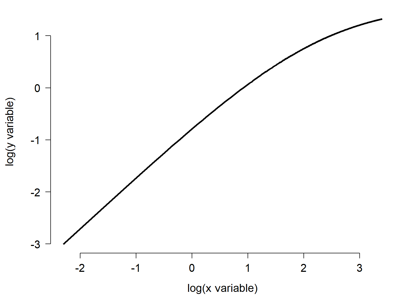
The function shown in Figure 22.1 is the famous Michaelis-Menten function, often used for enzyme kinetics.

22.1 Curve terminology

Straight lines are easy to describe. They have an angle relative to the axes (the slope) and one point where they intersect the y-axis: the intercept. Both of these characteristics are parameters of a function. A function is an operation that assigns each value in one set to exactly one value in another set. In this case, the function assigns each value in \(x\) to one and only one expected \(y\) value (remember, a statistical model has a deterministic part that produces the expected value, and a stochastic part for describing the residual variation).

22.1.1 Domain and codomain

Because a statistical model describes a function, the straight line acquires two more characteristics. The domain of the function is the set of inputs accepted by the function. The codomain is the set of outputs (some older books call this the range, but that term is now considered ambiguous).

Figure 22.3 shows some data and a linear function fitted to them. The domain of the fitted function is the interval between the smallest and largest \(x\) values. Its codomain is the interval that spans all of the observed \(y\) values.

Figure 22.3: A linear function f(x) fit to data and its domain, codomain, and expected values.

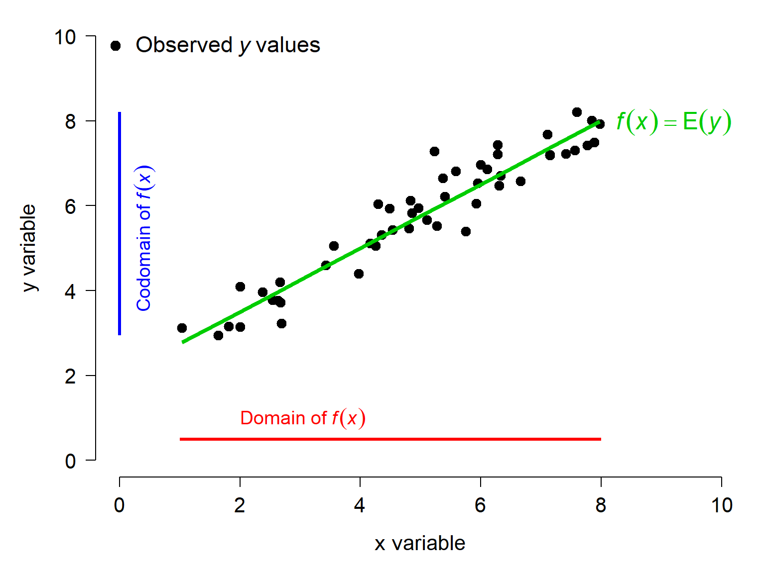
Mathematically, the domain and codomain of a linear function are the real numbers, often abbreviated \(\mathbb{R}\). But we’re not doing math, we are doing statistics. The linear model that we fit to the data is only applicable within the set of \(x\) and \(y\) values used to fit it. Using the model to make predictions outside the domain of its data, or extrapolation, can be fraught with peril.

22.1.2 Slopes and tangent lines

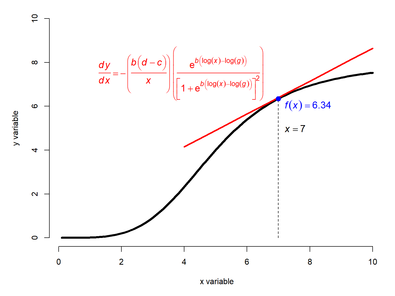
Nonlinear models, by definition, do not have a constant slope like a linear model does. Usually the slope of the function at any point is a function of the \(x\) value. Some of them have parameters that we refer to as a slope or growth rate, but these are really inputs to a function that determines the actual slope.

The function below shows a nonlinear curve \(f\left(x\right)\) and its tangent line at \(x=7\). The tangent line is a line that intersects a function at exactly one point and has the same slope as the function at that point. The slope of the tangent line is calculated as the first derivative of the function at that \(x\) value.

Figure 22.4: In this four-parameter log-logistic curve defined by parameters b, c, d, and g, the slope of the curve \(dy/dx\) at any point is not represented directly by any parameter but instead is a function of those parameters and \(x\). Here the slope at \(x=7\) is approximately \(0.749\).

22.1.3 Concavity

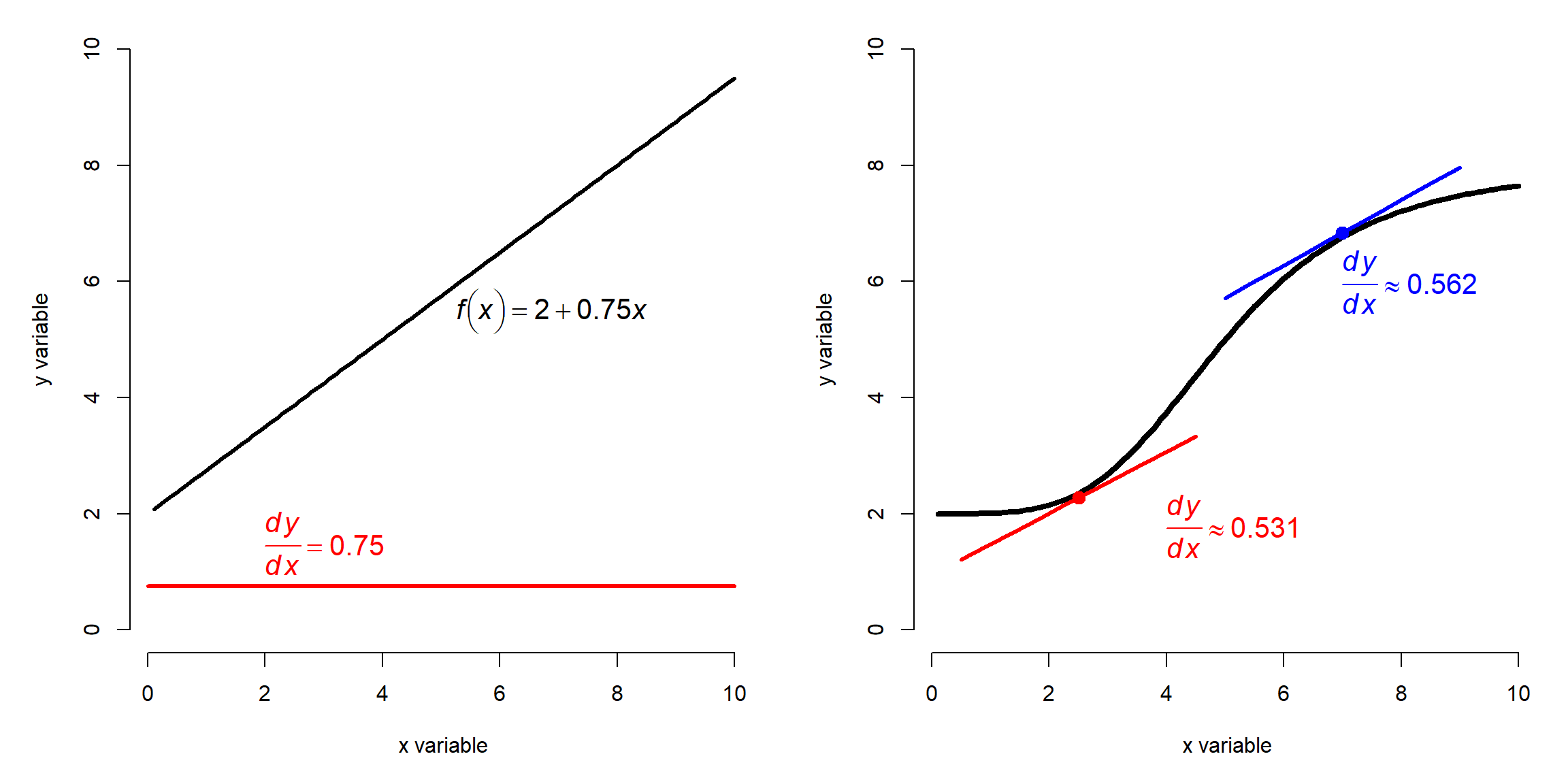
Nonlinear curves are also described by their concavity. A function is said to be concave up wherever its tangent line is below the graph of the function, and concave down when the tangent line lies above it. Remember the mnemonic, “up cup, down frown”. The concavity of a function is related to its second derivative, or the rate of change in the slope at any given point.

In Figure 22.5 below, the left panel shows a linear function \(y=2+0.75x\) and its constant slope of 0.75. The right panel shows a nonlinear curve whose slope changes with \(x\) (see Figure 22.4), and the tangent lines at \(x=2.5\) and \(x=7\). At the first point, the tangent line is below the function, so the function is concave up. At the second, the tangent line is above the function, so the function is concave down there. Note that the slopes of both tangent lines are positive.

Figure 22.5: Comparison of constant and variable slopes in linear and nonlinear functions. Left: A linear function has a constant first derivative (\(dy/dx = 0.75\)), represented by the horizontal red line. Right: A nonlinear sigmoidal function has a slope that changes with \(x\). Red and blue tangent lines illustrate the instantaneous slopes at two points along the curve, approximately 0.531 and 0.562, respectively.

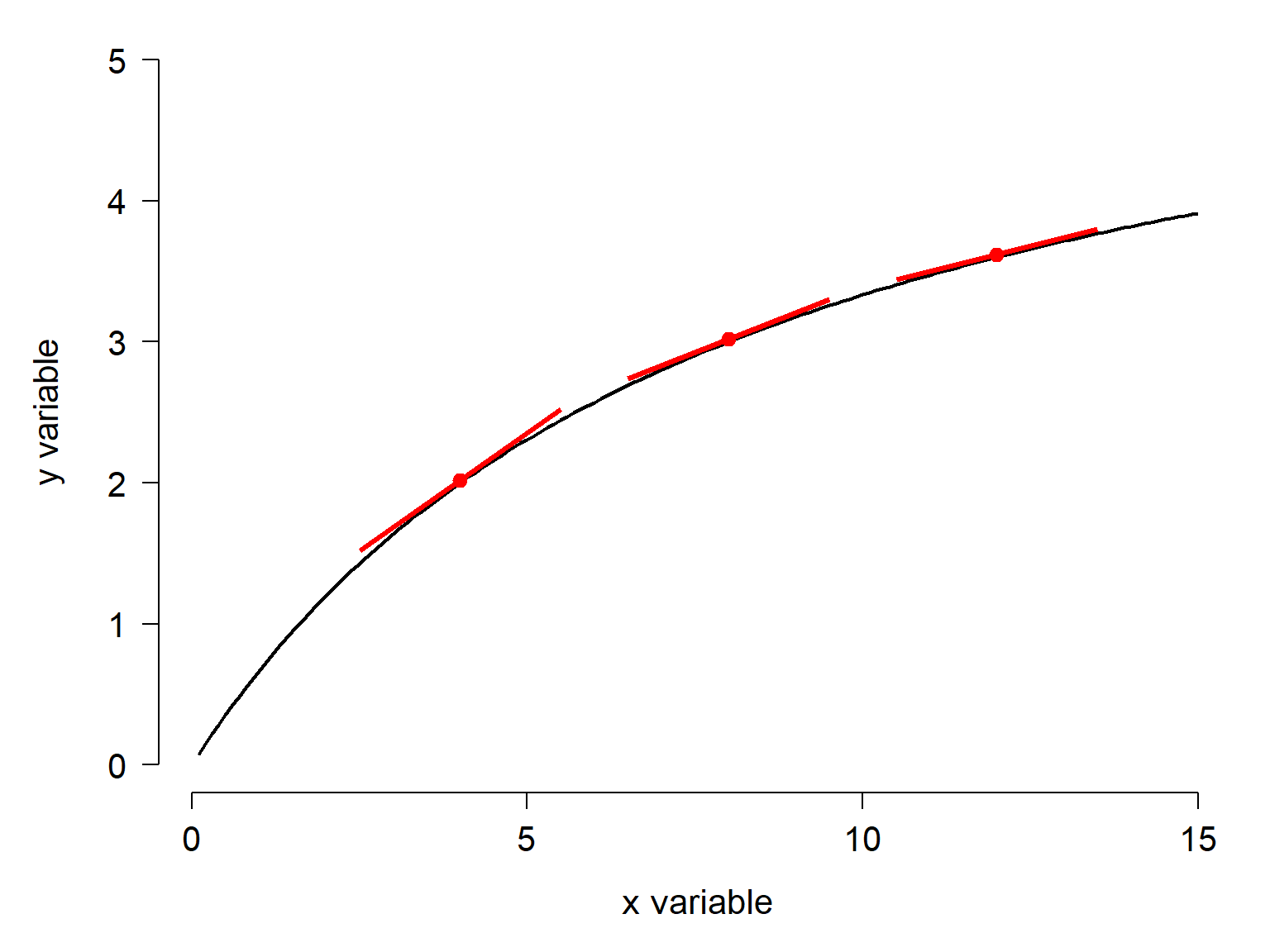
The second derivative that defines concavity is the rate of change in the slope: \(dy/dx/dx\), or \(dy/dx^2\). Figure 22.6 below shows a function which has a positive slope everywhere, but whose slope is decreasing. So, the function is concave down. Its first derivative is always positive, because the rate of change in \(y\) with respect to \(x\) is always positive, but that rate of change decreases as \(x\) gets larger.

Figure 22.6: The slope of this nonlinear function, represented by the red tangent lines, is always positive but decreases with increasing x.

22.1.4 Inflection points and midpoints

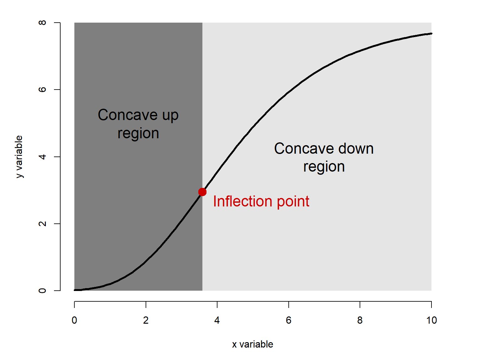
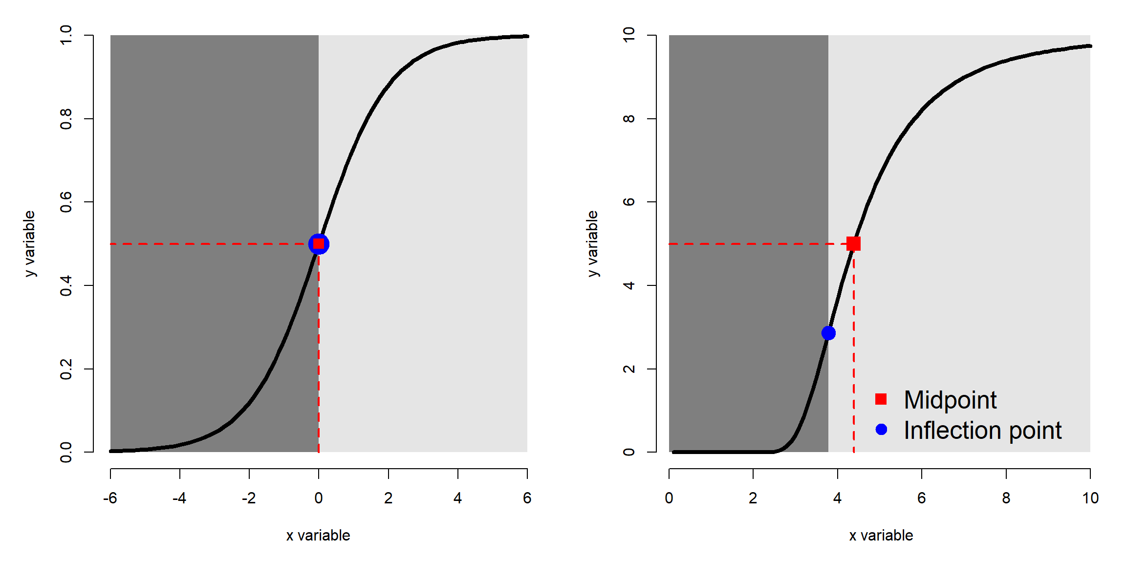
Some functions can change concavity over their domain. The \(x\) value at which they change concavity is called the inflection point. The function below has an inflection point near 3.6 where it changes from concave up (dark grey region) to concave down (light grey region). Some nonlinear functions have an inflection point as a parameter (Table 22.2).

Figure 22.7: Concavity and the inflection point of a nonlinear function. The curve is concave up in the darker shaded region, where its slope increases with \(x\) and the second derivative is positive. In the lighter shaded region, the curve is concave down, where its slope decreases with \(x\) and the second derivative is negative. The red point marks the inflection point, where the curve changes concavity and the second derivative equals zero.

When a function has a well-defined lower and upper value, we can define a midpoint: the \(x\) coordinate at which \(f\left(x\right)\) is equal to half of the distance between the minimum and the maximum. If the minimum is 0, then this is the \(x\) such that \(f\left(x\right)=\max{\left(f\left(x\right)\right)}/2\).

Figure 22.8: Parameters of the three-parameter log-logistic function. The parameter \(d\) determines the upper asymptote (blue dashed line), while \(g\) determines the midpoint of the curve along the \(x\)-axis. At \(x=g\), the response is halfway between the lower asymptote (zero) and the upper asymptote, so \(f(g)=d/2\). In this example, \(d=8\) and \(g=6\), giving \(f(6)=4\). The parameter \(b\) controls the steepness and direction of the curve.

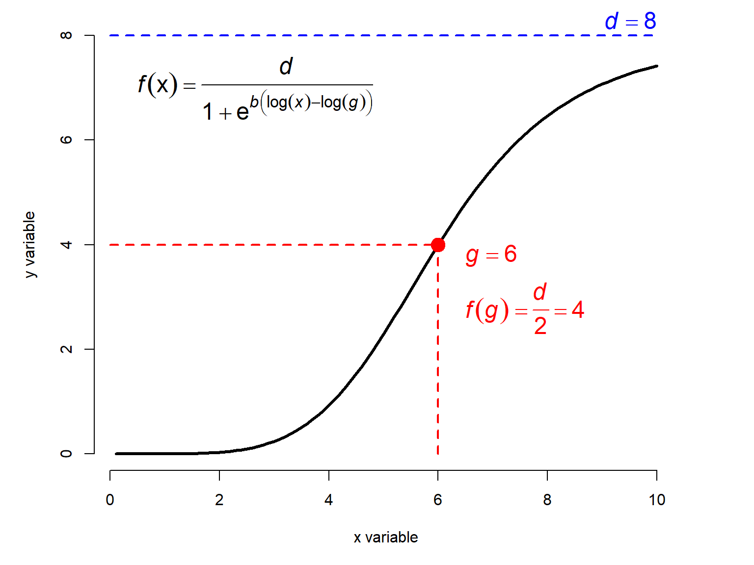
Note that although an inflection point and a midpoint may appear similar, they are not the same: an inflection point is where the concavity changes, and a midpoint is where the function has gone halfway from its minimum to its maximum. These can coincide, as in the standard logistic function in the left panel below, but more often they do not.

Figure 22.9: Comparison of the midpoint and inflection point in two sigmoidal functions. Left: In a symmetric sigmoid, the midpoint (red square) and inflection point (blue circle) coincide at the center of the curve, where the response is halfway between its asymptotes and the slope is greatest. Right: In an asymmetric sigmoid, the midpoint and inflection point occur at different values of \(x\). The inflection point marks the transition from concave up to concave down, while the midpoint identifies the response halfway between the asymptotes. Dark and light gray backgrounds indicate the concave-up and concave-down regions, respectively.

22.2 Common nonlinear functions

22.2.1 The Michaelis-Menten function

The Michaelis-Menten function is a nonlinear model that is usually used to describe processes that grow and approach an asymptote. One of the classic applications is modeling the relationship between biochemical reaction rates and substrate concentrations. The Michaelis-Menten equation takes the general form

\[Y=\frac{aX}{b+X}\]

where a and b are constants. It has a fixed lower bound at 0 and no inflection point.

• \(a\) is the asymptote: the maximum \(y\) value that is approached but never reached.
• \(b\) is the Michaelis constant. It represents the \(x\) value at which \(Y = a/2\). Interestingly, for any proportion of the form \(c/(c+1)\), where c is a positive integer, the X value where \(y=(c/(c+1))a\) is \(cb\). For example, the X value when \(y=(3/4)a\) is \(3b\).

x <- seq(0, 10, length=100)
a <- c(4, 6, 8, 10)
b <- 3

par(mfrow=c(2,1), mar=c(5,5,1,3), 
    xpd=NA, bty="n")
plot(x, x, type="n", xlab="x variable",
     ylab="y variable")
for(i in 1:length(a)){
    iy <- (a[i]*x)/(b+x)
    points(x, iy, type="l", lwd=3)
    text(max(x)+0.25, max(iy),
         paste("a =", a[i]),
         adj=0, cex=1.1)
}#i

a <- 5
b <- c(1, 3, 5, 7)
plot(x, x, type="n", xlab="x variable",
     ylab="y variable", ylim=c(0, 5))
for(i in 1:length(b)){
    iy <- (a*x)/(b[i]+x)
    points(x, iy, type="l", lwd=3)
    text(max(x)+0.25, max(iy),
         paste("b =", b[i]),
         adj=0, cex=1.1)
}#i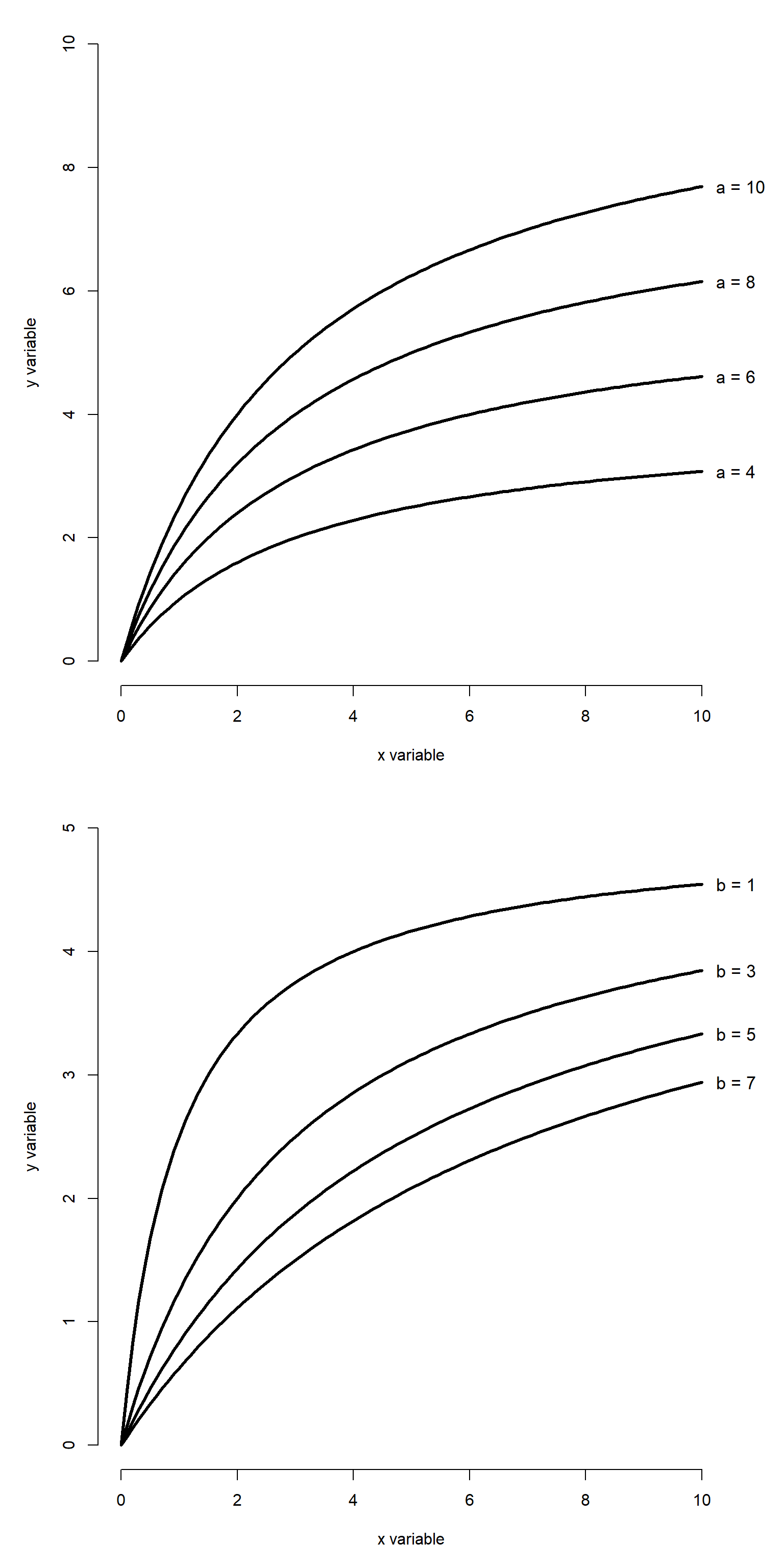

Figure 22.10: Top: Michaelis-Menten curves with fixed \(b\) and different asymptote (\(a\)) terms. Bottom: Michaelis-Menten curves with fixed \(a\) and different midpoints (\(b\)) terms

The Michaelis-Menten curve goes by many names. In enzyme kinetics and biochemistry, it is called the Michaelis-Menten curve. Biologists also sometimes call it the Monod function, the Holling type II functional response, or the Beverton-Holt model. This diversity of application speaks to the generality of this function. The original definition predicted a reaction rate. However, Michaelis-Menten curves can also be used to model other phenomena. For example, Kunz et al. (2019) and Green et al. (2020) used Michaelis-Menten curves to model the effectiveness of biodiversity monitoring programs, using the asymptote term as an estimate of the maximum number of species likely to be detected.

22.2.2 Gompertz functions

The Gompertz curve is a sigmoid (s-shaped) growth curve frequently used to describe biological growth. It can be written in several ways. You can use whichever form you want, but you need to be explicit about what you did. In both cases, all parameters must be positive.

22.2.2.1 Gompertz curve form 1

The most common form of the Gompertz curve is a double exponential:

\[\mathcal{f}\left(x\right)={ae}^{-be^{-cx}}\]

where \(a\) is the upper asymptote, \(b\) defines the x coordinate of the inflection point at \(\log{\left(b\right)/c}\), and \(c\) is a growth rate. The inflection point occurs at

\[x_{inflection}=\frac{\log\left(b\right)}{c}\]

and at that point,

\[y_{inflection}=\mathcal{f}\left(x_{inflection}\right)=\frac{a}{e}\approx0.368\]

22.2.2.2 Gompertz curve form 2

Another form of the Gompertz function looks like this:

\[\mathcal{f}\left(x\right)=ae^{-bc^x}\]

This version is used in the R SSgompertz function that we’ll see later. It is actually equivalent to the first version because of the identity

\[e^{-cx}=\left(e^{-c}\right)^x\]

Start with form 1 and substitute:

\[\mathcal{f}\left(x\right)={ae}^{-be^{-cx}}\]

\[\mathcal{f}\left(x\right)={ae}^{-b\left(e^{-c}\right)^x}\]

The second form replaces \(e^{-c}\) with a new constant, which the SSgompertz documentation calls b3 (with the \(b\) term from form 1 being renamed b2):

\[\mathcal{f}\left(x\right)={ae}^{-b_2\left(b_3\right)^x}\]

So, the two forms seen here produce the same curve, just in a slightly different way:

Table 22.1: Comparison of parameterizations of the Gompertz growth curve. The two equations describe the same curve, with the relationship \(b_3=e^{-c}\) (or equivalently, \(c=-\ln b_3\)).

Parameter	Classical: \(y=ae^{-be^{-cx}}\)	R SSgompertz(): \(y=ae^{-b_2b_3^x}\)	Interpretation
Upper asymptote	\(a\)	\(a\)	Maximum value approached as \(x\to\infty\).
Initial condition	\(b\)	\(b_2=b\)	Controls the initial value and horizontal position of the curve. At \(x=0\), \(y=ae^{-b}\).
Growth rate	\(c\)	\(b_3=e^{-c}\)	Controls how rapidly the curve approaches the asymptote. For increasing growth, \(c>0\) and \(0<b_3<1\).

Below is an illustration of the classic Gompertz curve with different parameters.

x <- seq(0, 10, length=100)
A <- c(4, 6, 8, 10)
B <- 3
C <- 2

par(mfrow=c(1,1), mar=c(5,5,1,3), 
    xpd=NA, bty="n")
plot(x, x, type="n", xlab="x variable",
     ylab="y variable", ylim=c(0, max(A)))
for(i in 1:length(A)){
    iy <- A[i]*exp(-1*B*exp(-1*C*x))
    points(x, iy, type="l", lwd=3)
    text(max(x)+0.25, max(iy),
         paste("a =", A[i]),
         adj=0, cex=1.1)
}#i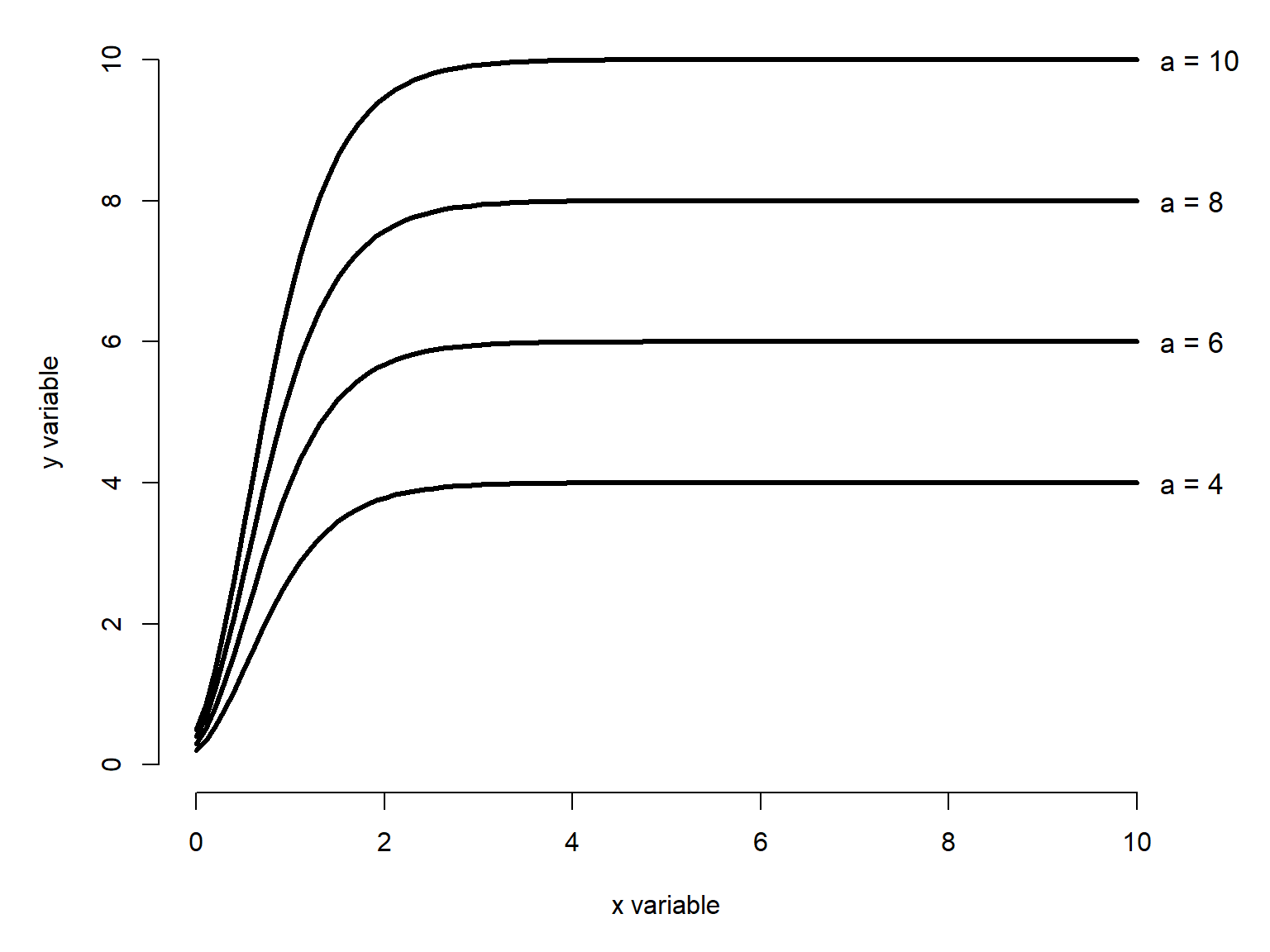

Figure 22.11: Gompertz growth curves with different asymptotes (\(a\)) and constant \(b\) and \(c\) parameters.

x <- seq(0, 10, length=100)
A <- 8
B <- c(3, 6, 9)
C <- 0.5
cols <- c("#e41a1c", "#377eb8", "#4daf4a")
par(mfrow=c(1,1), mar=c(5,5,1,3), 
    xpd=NA, bty="n")
plot(x, x, type="n", xlab="x variable",
     ylab="y variable", ylim=c(0, max(A)))
for(i in 1:length(B)){
    iy <- A*exp(-1*B[i]*exp(-1*C*x))
    points(x, iy, type="l", lwd=3,
           lty=i, col=cols[i])
}#i
legend("bottomright",
       legend=c(expression(italic(b)==3),
                expression(italic(b)==6),
                expression(italic(b)==9)),
       lty=1:3, lwd=3, col=cols,
       bty="n", cex=1.2)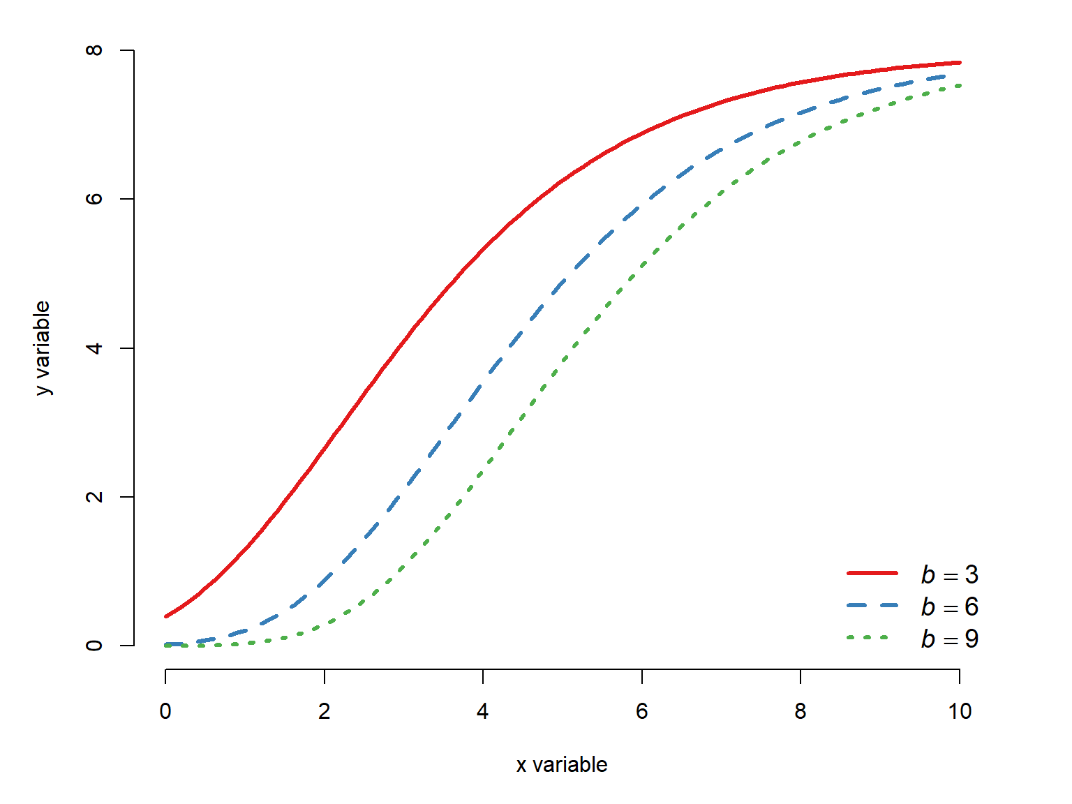

Figure 22.12: Gompertz growth curves with different \(b\) parameters, which control the horizontal displacement of the inflection point as \(\log{\left(b\right)}/c\). The \(a\) and \(c\) are held constant.

x <- seq(0, 10, length=100)
A <- 8
B <- 10
C <- c(0.25, 0.5, 1, 1.5)
cols <- c("#e41a1c", "#377eb8", "#4daf4a","#984ea3")
par(mfrow=c(1,1), mar=c(5,5,1,3), 
    xpd=NA, bty="n")
plot(x, x, type="n", xlab="x variable",
     ylab="y variable", ylim=c(0, max(A)))
for(i in 1:length(C)){
    iy <- A*exp(-1*B*exp(-1*C[i]*x))
    points(x, iy, type="l", lwd=3,
           lty=i, col=cols[i])
}#i
legend("bottomright",
       legend=c(expression(italic(c)==0.25),
                expression(italic(c)==0.5),
                expression(italic(c)==1),
                expression(italic(c)==1.5)),
       lty=1:3, lwd=3, col=cols,
       bty="n", cex=1.2)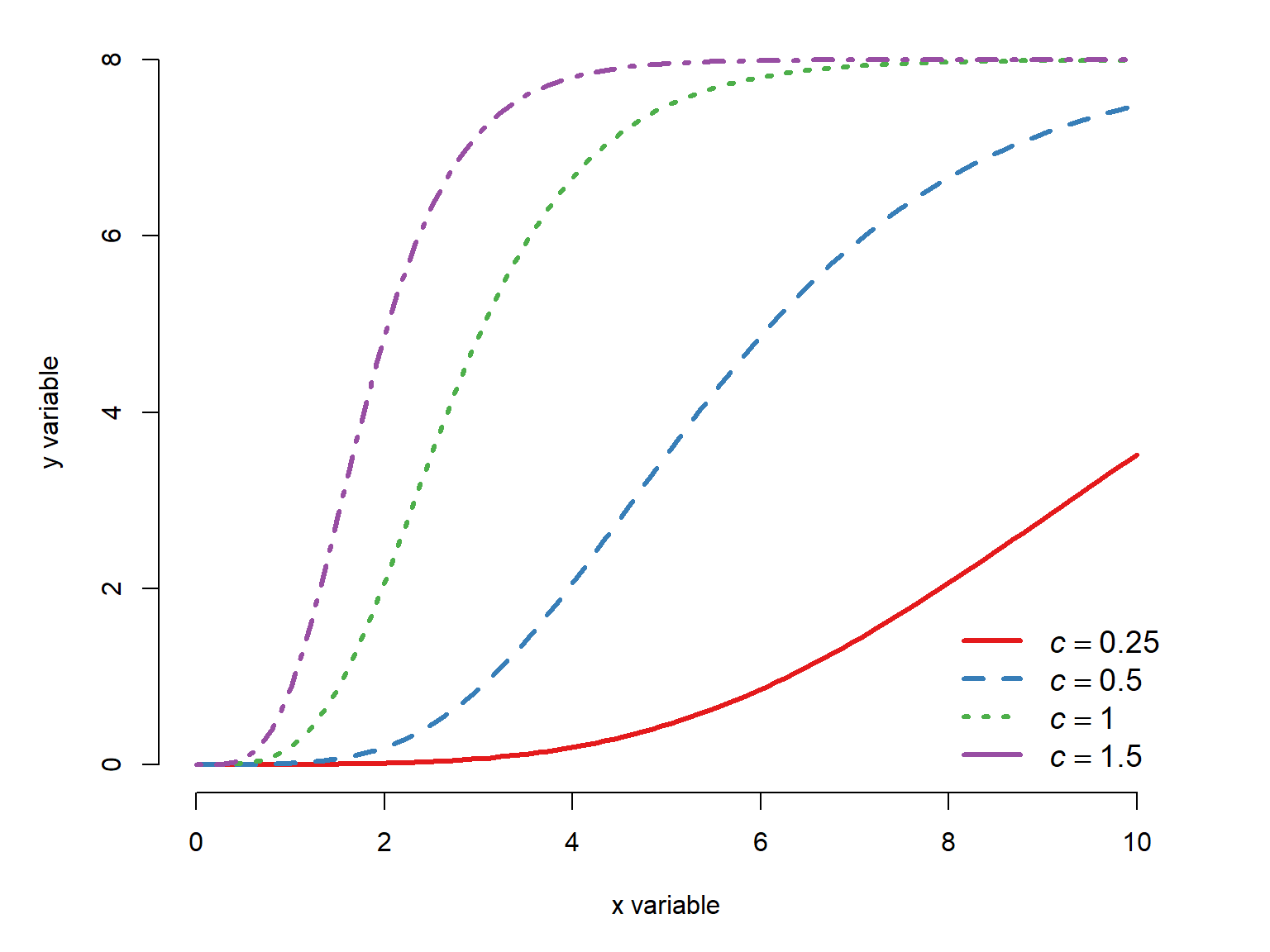

Figure 22.13: Gompertz growth curves with different \(c\) parameters, which control the growth rate of the curve. The \(a\) and \(b\) parameters are held constant.

22.2.3 The von Bertalanffy growth function

Like the Gompertz curve, the von Bertalanffy growth curve describes size increasing and approaching an asymptote. Unlike the Gompertz curve, the von Bertalanffy model is not sigmoid, but rather has a decreasing slope. That is, it is always concave down whereas the the Gompertz model can have a concave up portion, a concave down portion, and an inflection point in between.

The von Bertalanffy model is commonly written as:

\[f\left(x\right)=L_\infty\left(1-e^{-k\left(x-t_0\right)}\right)\]

where \(L_{\infty}\) is the asymptotic length as \(t\) approaches \(\infty\), \(k\) is a growth rate parameter, and \(t_0\) is the theoretical time at which \(\mathcal{f}\left(t\right)=0\). \(L_{\infty}\) and \(k\) must be positive, and \(t_0\) must be negative. The von Bertalanffy model is commonly used to describe animal growth, but in principle it could be used for any situation where its parameters make sense. The same function is also sometimes called the monomolecular curve. Like the Gompertz curve, the von Bertalanffy model has several forms. The form given above is the most common.

x <- seq(0, 50, length=100)
Linf <- c(50, 100, 150, 200)
K <- 0.05
T0 <- -1

C <- c(0.25, 0.5, 1, 2)
cols <- c("#e41a1c", "#377eb8", "#4daf4a","#984ea3")
par(mfrow=c(1,1), mar=c(5,5,1,4), 
    xpd=NA, bty="n")
plot(x, x, type="n", xlab="x variable",
     ylab="y variable", ylim=c(0, max(Linf)))
for(i in 1:length(Linf)){
    iy <- Linf[i]*(1-exp((-1*K)*(x-T0)))
    points(x, iy, type="l", lwd=3,
           lty=i, col=cols[i])
    text(max(x)+1, max(iy),
         bquote(italic(L)[infinity]==.(Linf[i])),
         adj=0, cex=1.2)
}#i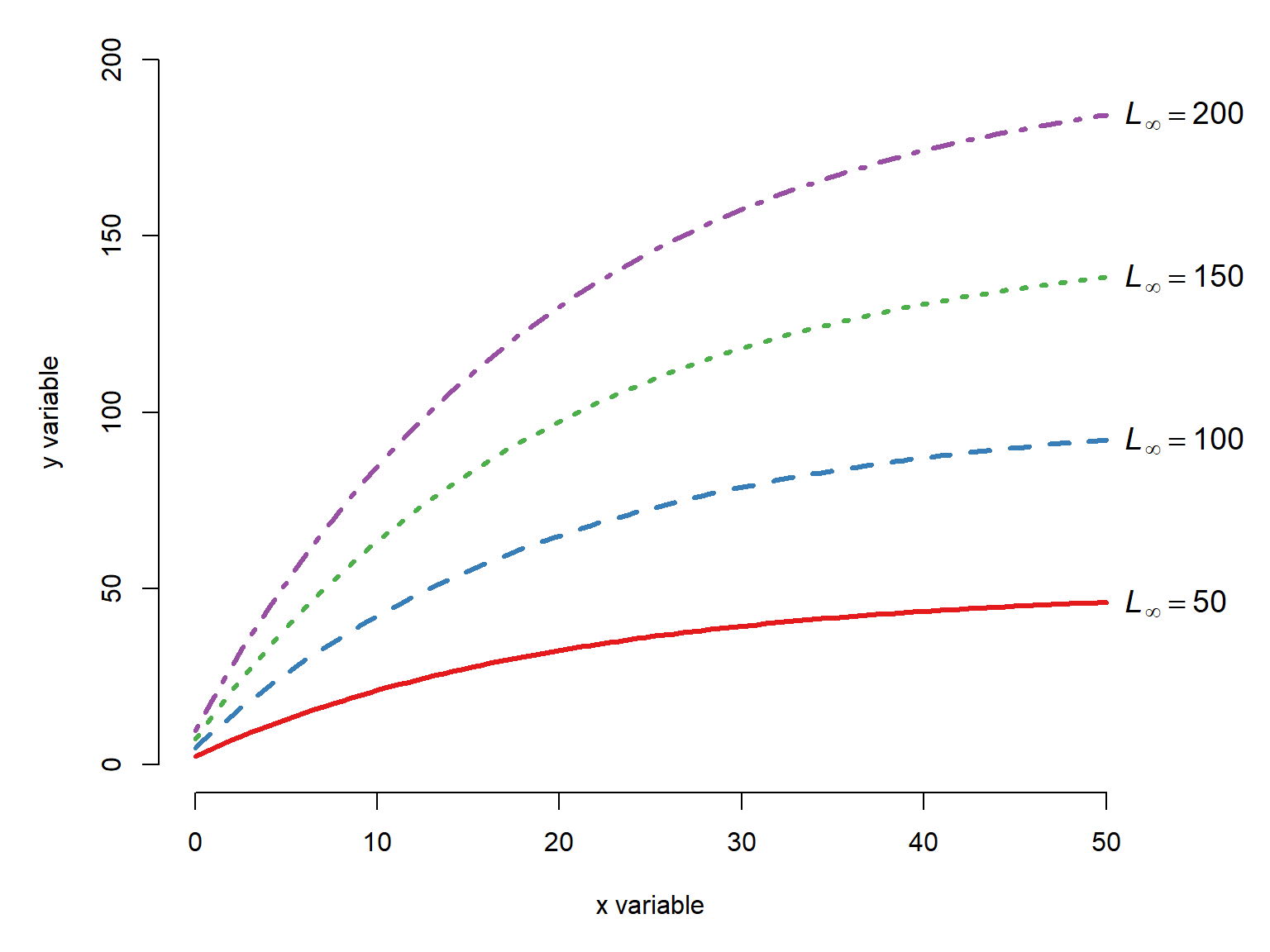

Figure 22.14: von Bertalanffy growth curves with different \(L_{\infty}\) parameters, which control maximal size (horizontal asympotote). The \(k\) and \(t_0\) parameters are held constant.

x <- seq(0, 50, length=100)
Linf <- 200
K <- c(0.01, 0.03, 0.05, 0.1)
T0 <- -1

cols <- c("#e41a1c", "#377eb8", "#4daf4a","#984ea3")
par(mfrow=c(1,1), mar=c(5,5,1,4), 
    xpd=NA, bty="n")
plot(x, x, type="n", xlab="x variable",
     ylab="y variable", ylim=c(0, max(Linf)))
for(i in 1:length(K)){
    iy <- Linf*(1-exp((-1*K[i])*(x-T0)))
    points(x, iy, type="l", lwd=3,
           lty=i, col=cols[i])
    text(max(x)+1, max(iy),
         bquote(italic(k)==.(K[i])),
         adj=0, cex=1.2)
}#i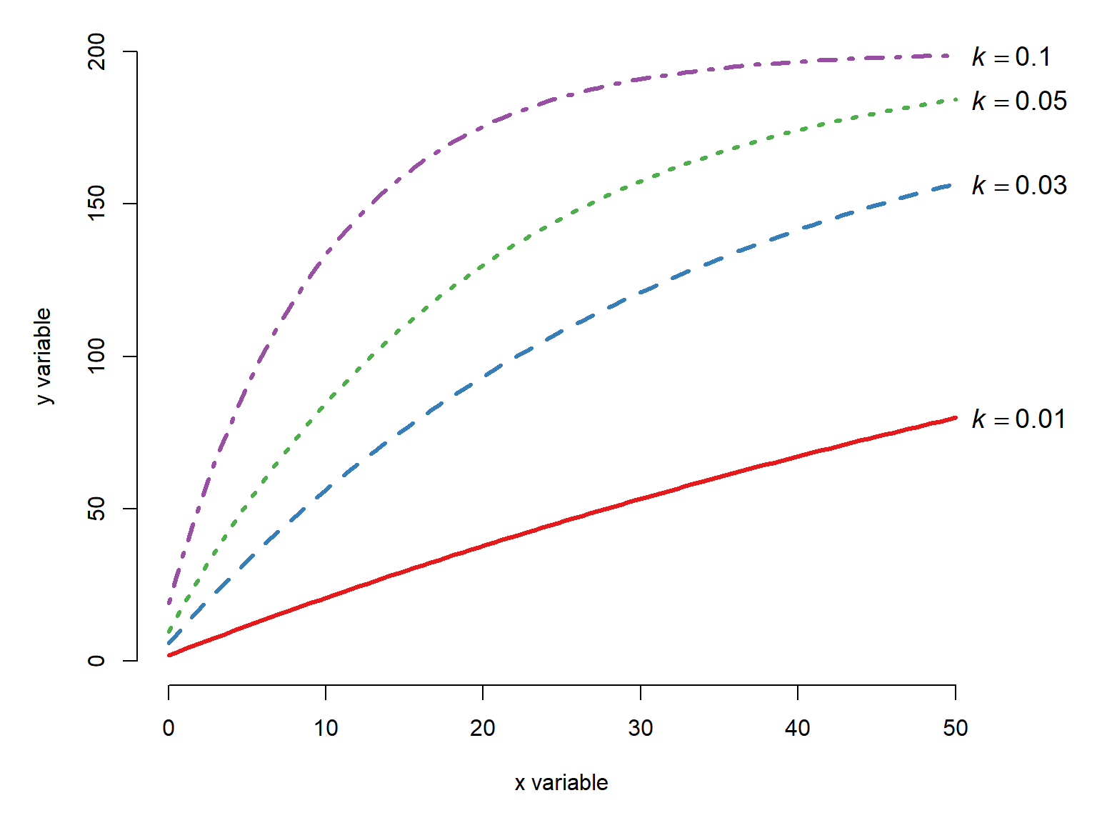

Figure 22.15: von Bertalanffy growth curves with different \(k\) parameters, which control growth rate. The \(L_{\infty}\) and \(t_0\) parameters are held constant.

x <- seq(0, 50, length=100)
Linf <- 200
K <- 0.05
T0 <- c(-1, -5, -10, -20)

cols <- c("#e41a1c", "#377eb8", "#4daf4a","#984ea3")
par(mfrow=c(1,1), mar=c(5,5,1,4), 
    xpd=NA, bty="n")
plot(x, x, type="n", xlab="x variable",
     ylab="y variable", ylim=c(0, max(Linf)))
for(i in 1:length(T0)){
    iy <- Linf*(1-exp((-1*K)*(x-T0[i])))
    points(x, iy, type="l", lwd=3,
           lty=i, col=cols[i])
}#i
legend("bottomright",
       legend=c(expression(italic(t)[0]==-1),
                expression(italic(t)[0]==-5),
                expression(italic(t)[0]==-10),
                expression(italic(t)[0]==-20)),
       lty=1:3, lwd=3, col=cols,
       bty="n", cex=1.2)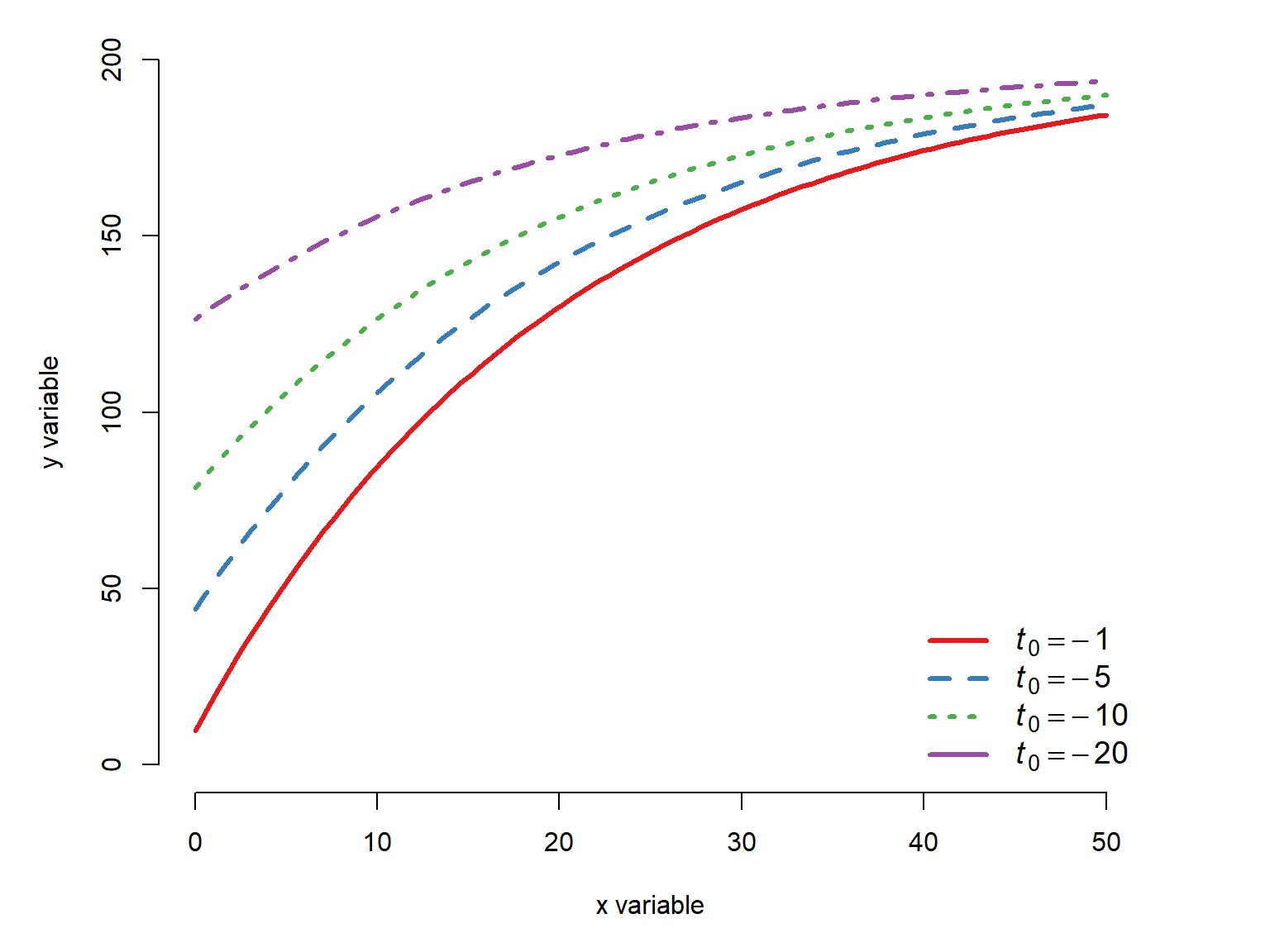

Figure 22.16: von Bertalanffy growth curves with different \(t_0\) parameters, which control horizontal displacement and the y-intercept. The \(L_{\infty}\) and \(k\) parameters are held constant.

22.2.4 Logistic and log-logistic functions

A logistic curve is one that takes the form

\[f\left(x\right)=\frac{L}{1+e^{-b\left(x-x_0\right)}}\]

where \(L\) is the supremum (upper asymptote), \(b\) is a growth rate, and \(x_0\) is the midpoint (\(x\) value where \(f\left(x\right)=L/2\)). Logistic functions are sigmoid, with a lower limit of 0 as x tends to \(-\infty\) and upper limit of \(L\) as x approaches \(+\infty\). The standard logistic function with \(L=1\), \(b=1\) and \(x_0=0\) is

\[f\left(x\right)=\frac{1}{1+e^{-x}}\]

which you may recognize as the inverse of the logit function, given by the R function plogis().

x <- seq(-6, 6, length=100)
y <- plogis(x)

par(mfrow=c(1,1), mar=c(5,5,1,3), 
    xpd=NA, bty="n")
plot(x, y, type="l", lwd=3, xlab="x variable",
     ylab="y variable", ylim=c(0, 1))
segments(0, 0, 0, 0.5, lty=2, lwd=2, col="red")
segments(0, 0.5, -6, 0.5, lty=2, lwd=2, col="red")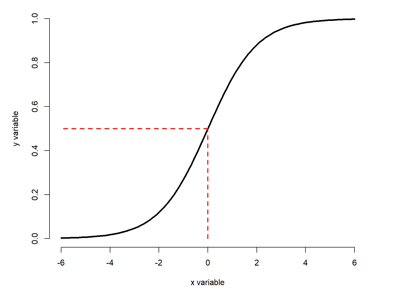

Figure 22.17: The standard logistic curve \(f\left(x\right)=1/\left(1+e^{-x}\right)\). The red dashed line illustrates how the inflection point and midpoint are at \(x=0\)

The logistic function can be generalized by adding parameters to specify the upper and lower asymptotes or other features. These versions are called log-logistic functions because they use the logarithm of \(x\), not \(x\) itself. We will examine four versions:

• the two-parameter log-logistic (2pl): uses a midpoint (\(g\)) and a slope parameter (\(b\)), with lower and upper asymptotes fixed at 0 and 1, respectively.
• the three-parameter log-logistic (3pl): extends the two-parameter log-logistic model with a new term \(d\) to define an upper asymptote other than 1.
• the four-parameter log-logistic (4pl): extends the three-parameter log-logistic model with a new term \(c\) to define a lower asymptote other than 0.
• the five-parameter log-logistic (5pl): extends the four-parameter log-logistic model with a new term \(h\) to alter the shape of the curve.

In practical terms:

• the four-parameter model is just the special case of the five-parameter model with \(h=1\)
• the three-parameter model is just the special case of the four-parameter model with \(c=0\)
• the two-parameter model is the special case of the three-parameter model with \(d=1\).

NoteA note on parameter names

Textbooks and software packages differ a bit in the way that they label the parameters of the models in this section. In this guide I have tried to be as consistent as possible, at least within each group like the log-logistic or the Weibull families. The letters or symbols are not important–their positions in the equations are. In general, I try to avoid using \(e\) and \(f\) as names of parameters because in most contexts \(e\) is the symbol for Euler’s number and \(f\) is often used to label functions (e.g., \(f\left(x\right)=\dots\)).

22.2.4.1 Two-parameter log-logistic

The two-parameter log-logistic function is like the standard logistic function (Figure 22.17), but with parameters \(b\) for the slope and \(g\) for the midpoint. It is given by:

\[f\left(x\right)=\frac{1}{1+e^{b\left(\log{\left(x\right)}-\log{\left(g\right)}\right)}}\]

Notice that here \(x\) is part of a difference in the exponent, which has the effect of moving the curve left and right.

The \(b\) parameter defines the curve’s growth rate. Counter intuitively, the function increases when \(b<0\), and decreases when \(b>0\). Greater magnitudes of \(b\), regardless of sign, make for steeper curves.

x <- seq(0.1, 10, length=100)
B <- -1*c(0.5, 1, 2, 4, 8)
G <- 5

cols <- c("#e41a1c", "#377eb8", "#4daf4a","#984ea3", "#ff7f00")
par(mfrow=c(1,1), mar=c(5,5,1,4), 
    xpd=NA, bty="n")
plot(x, x, type="n", xlab="x variable",
     ylab="y variable", ylim=c(0, 1))
for(i in 1:length(B)){
    iy <- 1/(1+exp(B[i]*(log(x)-log(G))))
    points(x, iy, type="l", lwd=3,
           lty=i, col=cols[i])
    text(max(x)+0.2, max(iy),
         bquote(italic(b)==.(B[i])),
         adj=0, cex=1.2,
         col=cols[i])
}#i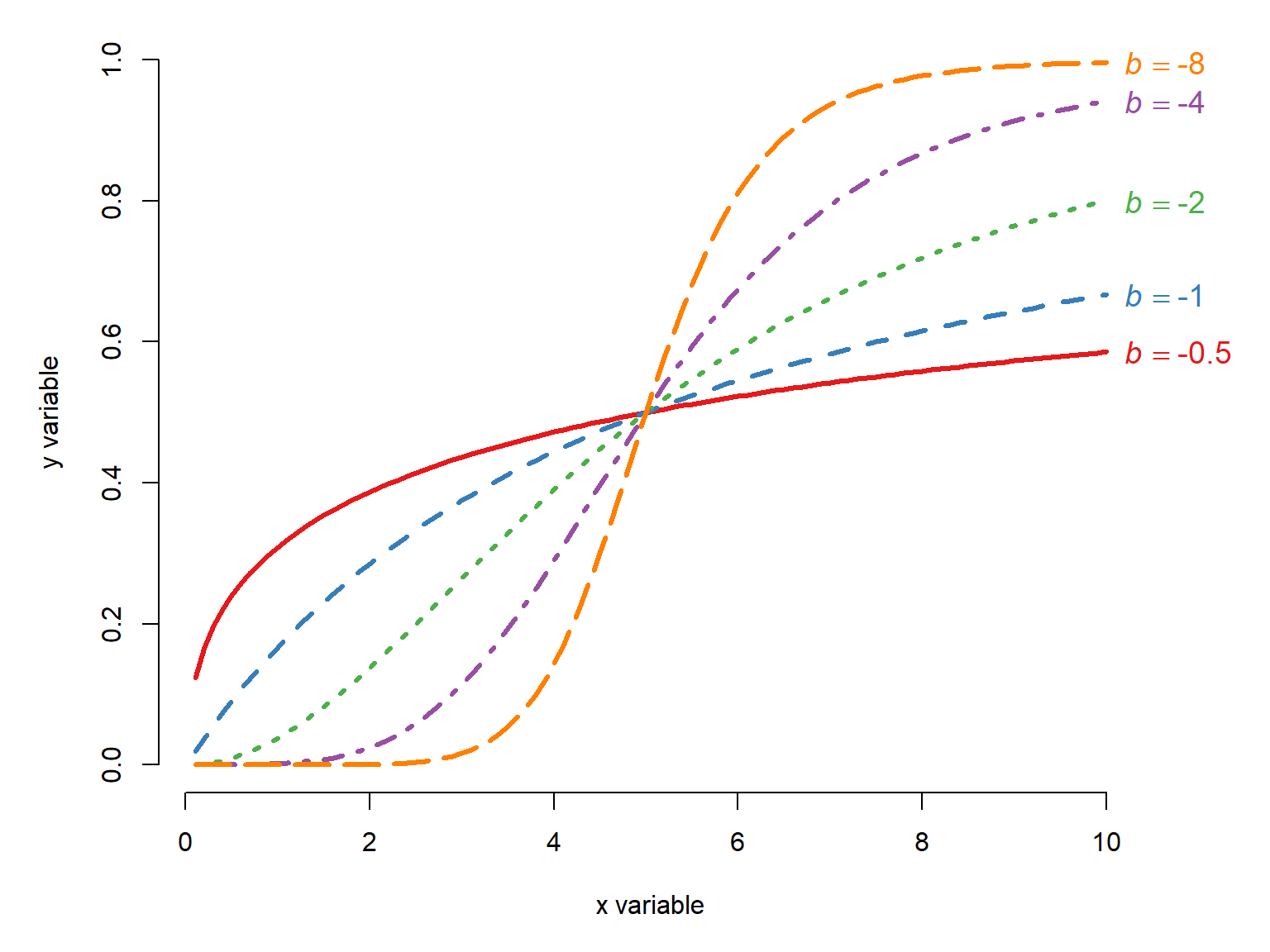

Figure 22.18: Two-parameter log-logistic curves with different \(b\) parameters, which control the growth rate. Negative \(b\) of greater magnitude cause faster growth. The midpoint parameter \(g\) is constant at 5$.

Positive \(b\) cause the function to decrease:

x <- seq(0.1, 10, length=100)
B <- c(0.5, 1, 2, 4, 8)
G <- 5

cols <- c("#e41a1c", "#377eb8", "#4daf4a","#984ea3", "#ff7f00")
par(mfrow=c(1,1), mar=c(5,5,1,4), 
    xpd=NA, bty="n")
plot(x, x, type="n", xlab="x variable",
     ylab="y variable", ylim=c(0, 1))
for(i in 1:length(B)){
    iy <- 1/(1+exp(B[i]*(log(x)-log(G))))
    points(x, iy, type="l", lwd=3,
           lty=i, col=cols[i])
}#i
legend("topright", 
       legend=c(
           expression(italic(b)==0.5),
           expression(italic(b)==1),
           expression(italic(b)==2),
           expression(italic(b)==4),
           expression(italic(b)==8)),
       bty="n", cex=1.2,
       lty=1:5, col=cols, lwd=3)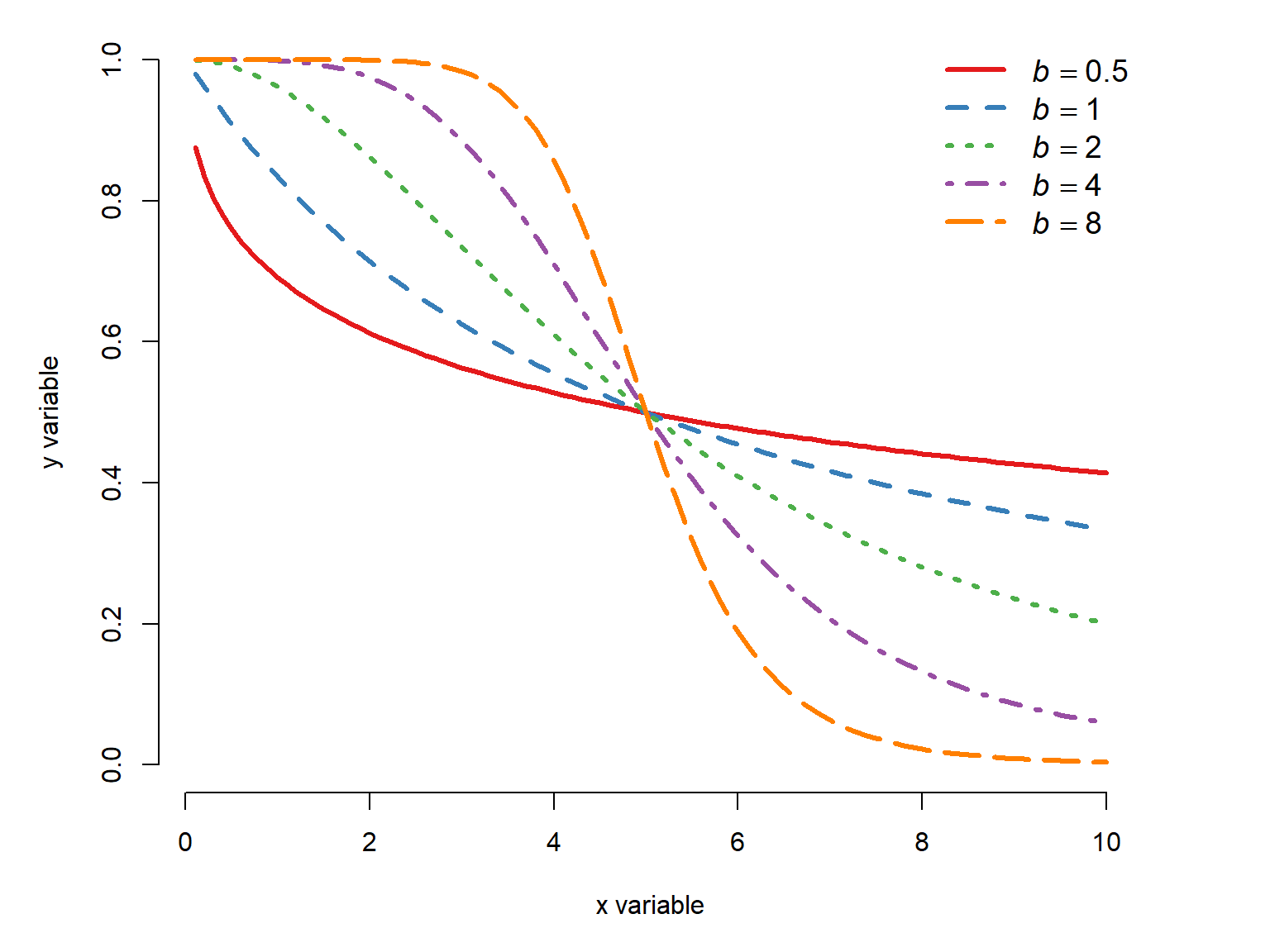

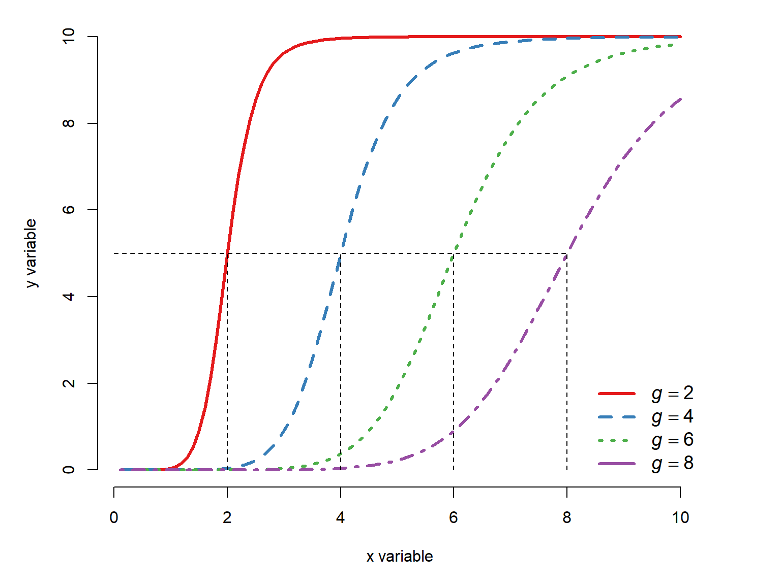
Figure 22.19: Two-parameter log-logistic curves with different \(b\) parameters, which control the growth rate. Positive \(b\) of greater magnitude cause faster decay. The midpoint parameter \(g\) is constant at 5$.

The \(g\) parameter defines the midpoint, or \(x\) value at which \(y=1/2\).

x <- seq(0.1, 10, length=100)
B <- -5
G <- c(2, 4, 6, 8)

cols <- c("#e41a1c", "#377eb8", "#4daf4a","#984ea3")
par(mfrow=c(1,1), mar=c(5,5,1,4), 
    xpd=NA, bty="n")
plot(x, x, type="n", xlab="x variable",
     ylab="y variable", ylim=c(0, 1))
for(i in 1:length(G)){
    iy <- 1/(1+exp(B*(log(x)-log(G[i]))))
    points(x, iy, type="l", lwd=3,
           lty=i, col=cols[i])
}#i
legend("bottomright", 
       legend=c(
           expression(italic(g)==2),
           expression(italic(g)==4),
           expression(italic(g)==6),
           expression(italic(g)==8)),
       bty="n", cex=1.2,
       lty=1:5, col=cols, lwd=3)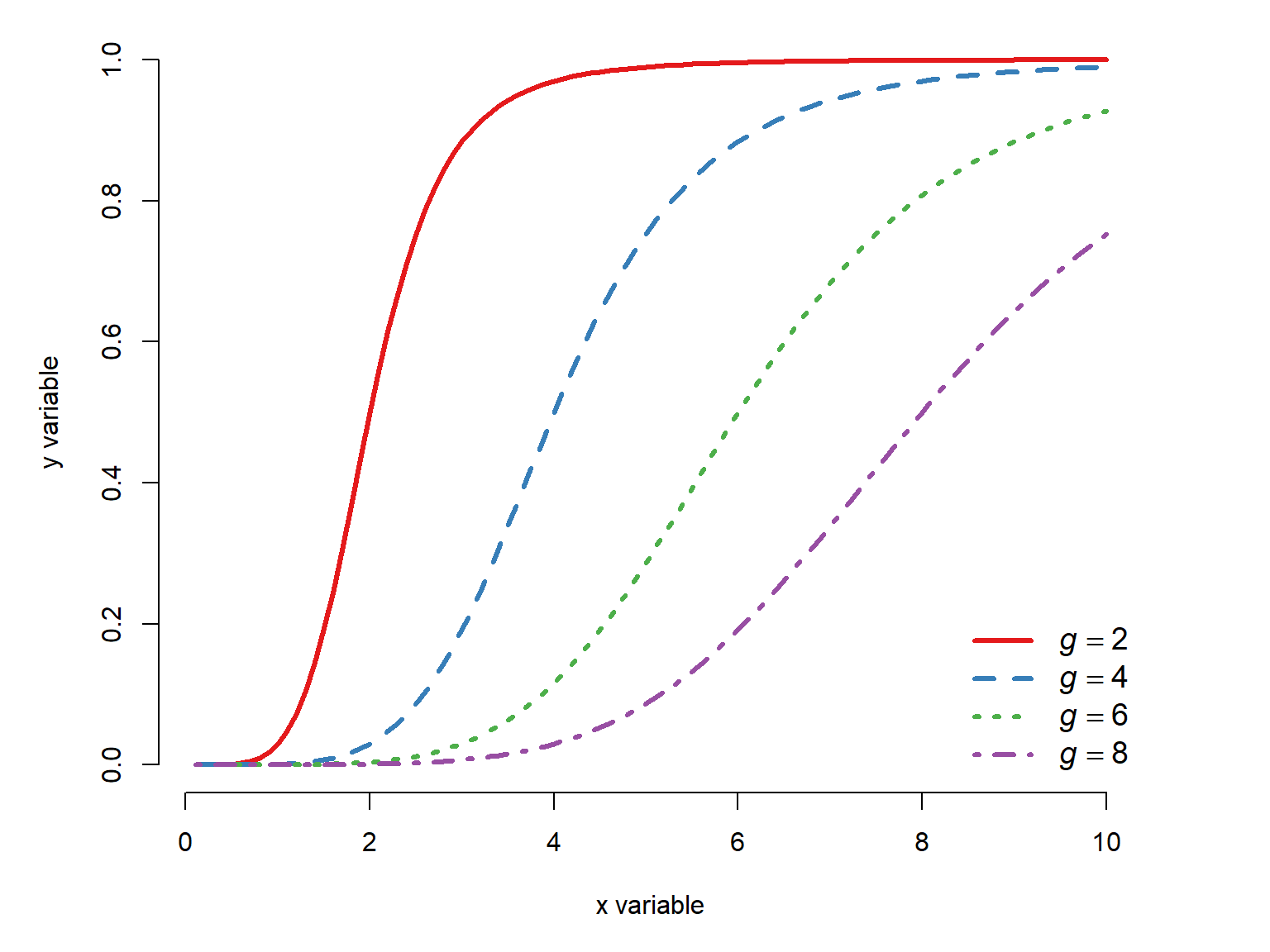

Figure 22.20: Two-parameter log-logistic curves with different \(g\) parameters, which control the function midpoint. Greater \(g\) shift the curve to the right. The \(b\) term is held constant at -5.

22.2.4.2 Three-parameter log-logistic

The three-parameter log-logistic generalizes the two-parameter log-logistic by adding a term for either the upper or lower asymptote. Either the lower limit is fixed at 0 and the upper limit is the parameter \(d\), or the upper limit can be fixed at 1 and the lower limit is the parameter \(c\). The former version, with lower limit fixed at 0, is probably more common so we’ll focus on that one.

Lower limit fixed at 0:

The most commonly encountered version of the three-parameter log-logistic model has the lower limit fixed at 0 and the upper limit as a parameter \(d\):

\[f\left(x\right)=\frac{d}{1+e^{b\left(\log{\left(x\right)}-\log{\left(g\right)}\right)}}\]

where \(d\) is the upper asymptote, \(b\) is a growth rate, and \(g\) is the inflection point.

Tipe is not always e

In the R documentation for log-logistic functions, especially in package drc, the midpoint parameter that we call \(g\) here is often referred to as \(e\). I find this incredibly unhelpful, so I use a different letter instead. Using \(e\) for something other than Euler’s constant is like using \(\pi\) to stand for something other than the ratio of a circle’s circumference to its diameter…which people also do sometimes. Read the documentation!

Upper limit fixed at 1:

The less commonly encountered version of the three-parameter log-logistic function has the upper limit fixed at 1 and the lower limit as a parameter \(c\):

\[f\left(x\right)=c+\frac{1-c}{1+e^{b\left(\log{\left(x\right)}-\log{\left(g\right)}\right)}}\]

Here is an illustration of the fixed-lower version of the three-parameter log-logistic function with differing upper asymptotes:

x <- seq(0.1, 10, length=100)
B <- -5
G <- 5
D <- c(4, 8, 12, 16)

cols <- c("#e41a1c", "#377eb8", "#4daf4a","#984ea3")
par(mfrow=c(1,1), mar=c(5,5,1,4), 
    xpd=NA, bty="n")
plot(x, x, type="n", xlab="x variable",
     ylab="y variable", ylim=c(0, max(D)))
for(i in 1:length(D)){
    iy <- D[i]/(1+exp(B*(log(x)-log(G))))
    points(x, iy, type="l", lwd=3,
           lty=i, col=cols[i])
    text(max(x)+0.2, max(iy),
         bquote(italic(d)==.(D[i])),
         adj=0, cex=1.2,
         col=cols[i])
}#i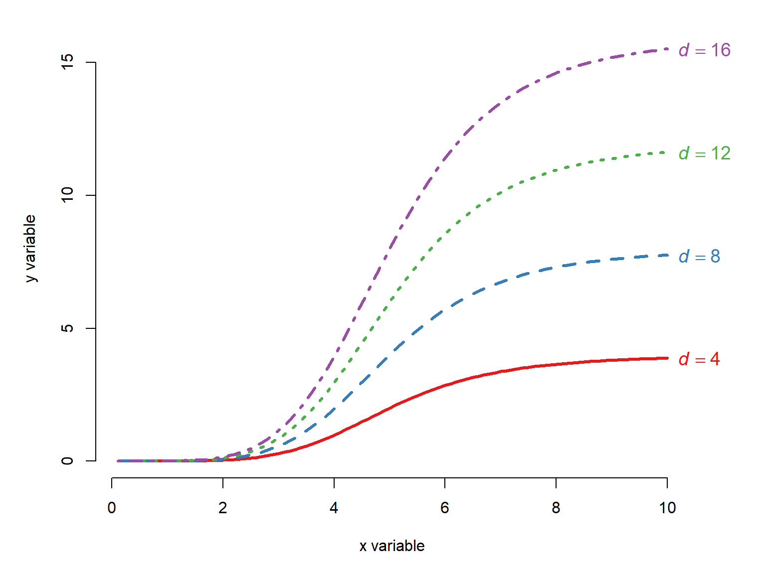

Figure 22.21: Three-parameter log-logistic curves with different \(d\) parameters, which control the upper asymptote. Greater \(d\) increase the maximal value of the curve. The other parameters are held constant at \(b=-4\) and \(g=5\).

If we hold \(d\) constant, then visualizing the effect of different \(b\) or \(g\) is exactly as it was in Figure 22.18 and Figure 22.19, just with a different upper value on the y-axis.

22.2.4.3 Four-parameter log-logistic

If we take the three-parameter log-logistic, and allow both the upper and lower asymptotes to vary, we get the four parameter log-logistic. It has terms for the lower asymptote (\(c\)), upper asymptote (\(d\)), midpoint (\(g\)), and growth rate (\(b\)):

\[f\left(x\right)=c+\frac{d-c}{1+e^{b\left(\log{\left(x\right)}-\log{\left(g\right)}\right)}}\]

As in all of these log-logistic curves, the \(g\) parameter is particularly useful because it can be interpreted as the ED50, or the dose producing a response halfway between \(c\) and \(d\). When \(c=0\) and \(d=1\), this is literally a response of 50% or 0.5; otherwise the \(g\) parameter relates to a response midway between \(c\) and \(d\). Again, note that what we are calling \(g\) is referred to in the drc documentation as e.

Here is an illustration of the four-parameter log-logistic curve with varying \(b\) parameters:

x <- seq(0.1, 10, length=100)
B <- -1*c(0.5, 1, 2, 4, 8)
C <- 0
D <- 10
G <- 5

cols <- c("#e41a1c", "#377eb8", "#4daf4a","#984ea3", "#ff7f00")
par(mfrow=c(1,1), mar=c(5,5,1,4), 
    xpd=NA, bty="n")
plot(x, x, type="n", xlab="x variable",
     ylab="y variable", ylim=c(0, max(D)))
for(i in 1:length(B)){
    iy <- C+(D-C)/(1+exp(B[i]*(log(x)-log(G))))
    points(x, iy, type="l", lwd=3,
           lty=i, col=cols[i])
    text(max(x)+0.2, max(iy),
         bquote(italic(b)==.(B[i])),
         adj=0, cex=1.2,
         col=cols[i])
}#i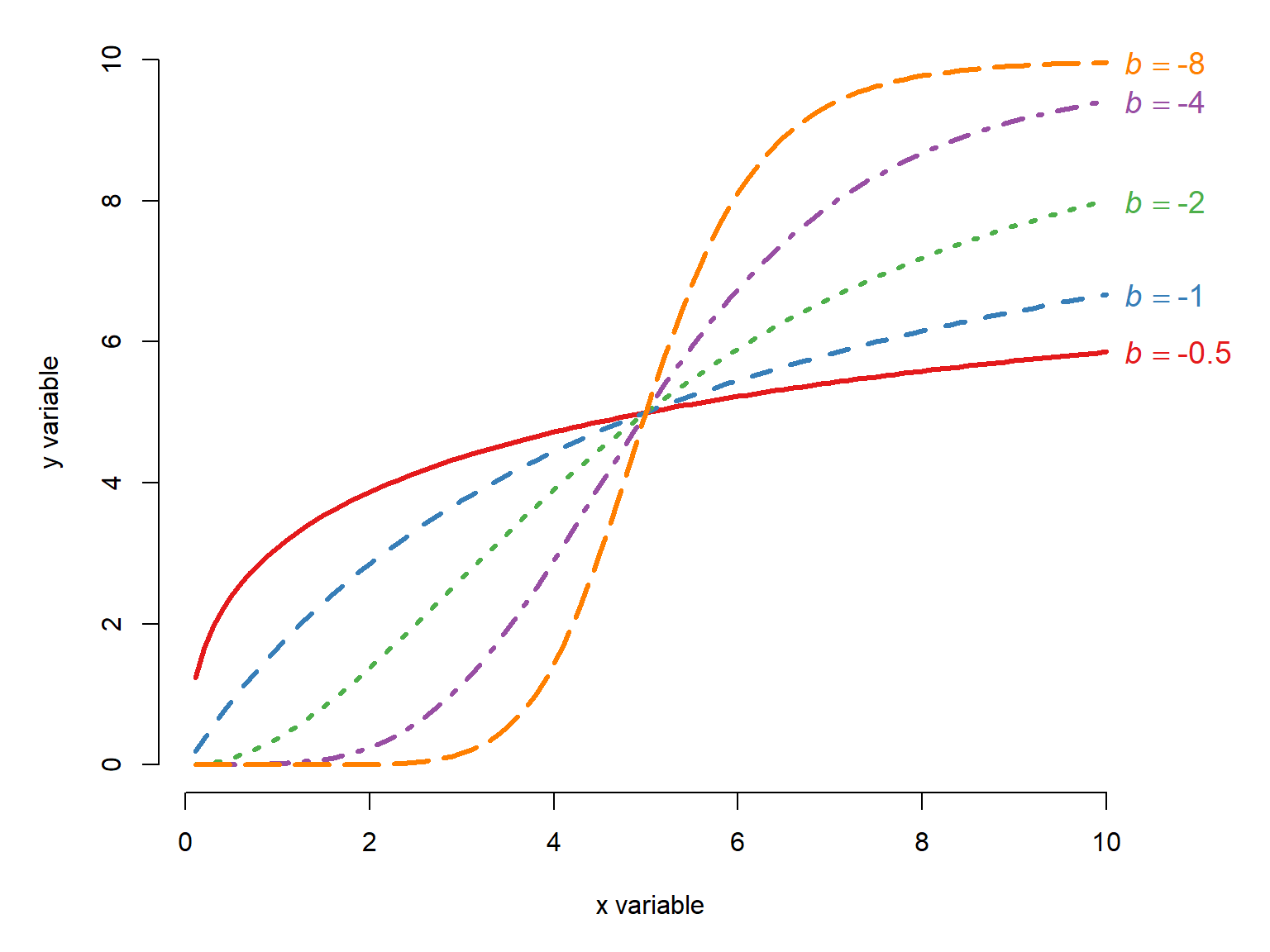

Figure 22.22: Four-parameter log-logistic curves with different \(b\) parameters, which control the growth rate. The other parameters are constant at \(c=0\), \(d=10\), and \(g=5\).

Here is an illustration of the four-parameter log-logistic curve with varying \(g\) parameters:

x <- seq(0.1, 10, length=100)
B <- -8
C <- 0
D <- 10
G <- c(2, 4, 6, 8)

cols <- c("#e41a1c", "#377eb8", "#4daf4a","#984ea3")
par(mfrow=c(1,1), mar=c(5,5,1,4), 
    xpd=NA, bty="n")
plot(x, x, type="n", xlab="x variable",
     ylab="y variable", ylim=c(0, max(D)))
for(i in 1:length(G)){
    iy <- C+(D-C)/(1+exp(B*(log(x)-log(G[i]))))
    points(x, iy, type="l", lwd=3,
           lty=i, col=cols[i])
}#i
legend("bottomright",
       legend=c(expression(italic(g)==2),
                expression(italic(g)==4),
                expression(italic(g)==6),
                expression(italic(g)==8)),
       lty=1:3, lwd=3, col=cols,
       bty="n", cex=1.2)
for(i in 1:length(G)){
    segments(0, D/2, G[i], D/2, lty=2)
    segments(G[i], 0, G[i], D/2, lty=2)
}

Figure 22.23: Four-parameter log-logistic curves with different \(g\) parameters, which control the growth rate and midpoint. The black dashed lines illustrate how the \(g\) parameter is really the \(x\) value where \(y=d/2\). The other parameters are constant at \(c=0\), \(d=10\), and \(b=-8\).

Varying the \(c\) and \(d\) terms in the four-parameter log-logistic move the lower and upper asymptotes, and correspondingly can squash or stretch the curves. See Figure 22.21 for an illustration of what that might look like.

22.2.4.4 Five-parameter log-logistic

The most flexible version of the log-logistic model has 5 parameters: a lower asymptote \(c\), an upper asymptote \(d\), a growth rate \(b\), a midpoint \(g\), and a shape parameter \(h\). When \(h\neq1\), the function is asymmetric about \(g\). When \(h=1\), the model reduces to the four-parameter log-logistic. We obtain the five-parameter model by adding an exponent \(h\) to the entire denominator of the four-parameter model :

\[f\left(x\right)=c+\frac{d-c}{\left(1+e^{b\left(\log{\left(x\right)}-\log{\left(g\right)}\right)}\right)^h}\]

The exponent \(h\) allows the curve to be asymmetric about the midpoint \(g\), when \(h\neq1\). For an intuition about what \(h\) does, imagine that the curve is a rubber or plastic rod bent into an s-shape–the shape of the log-logistic curve. If you grab the rod at the midpoint \(g\) and twist clockwise, the curve will decrease left of \(g\) and increase right of \(g\). That is like decreaseing \(h\) from 1 towards 0. If you twist counter-clockwise, the curve will decrease. This is like increasing \(h\) from 1. Note that we need to adjust \(g\) as a function of \(h\) to keep the midpoint the same.

x <- seq(1, 500, length=100)
B <- -2
C <- 0
D <- 10
G <- 150
H <- c(1, 0.75, 0.5, 0.25, 0.1)


cols <- c("black", "#e41a1c", "#377eb8", "#4daf4a","#984ea3")
par(mfrow=c(1,1), mar=c(5,5,1,4), 
    xpd=NA, bty="n")
plot(x, x, type="n", xlab="x variable",
     ylab="y variable", ylim=c(0, max(D)))
for(i in 1:length(H)){
    ig <- G / (2^(1/H[i])-1)^(1/B)
    iy <- C+(D-C)/((1+exp(B*(log(x)-log(ig))))^H[i])
    lines(x, iy, lwd=3, lty=i, col=cols[i])
}#i
legend("topleft",
       legend=c(expression(italic(h)==1),
                expression(italic(h)==0.75),
                expression(italic(h)==0.5),
                expression(italic(h)==0.25),
                expression(italic(h)==0.1)),
       lty=1:3, lwd=3, col=cols,
       bty="n", cex=1.2)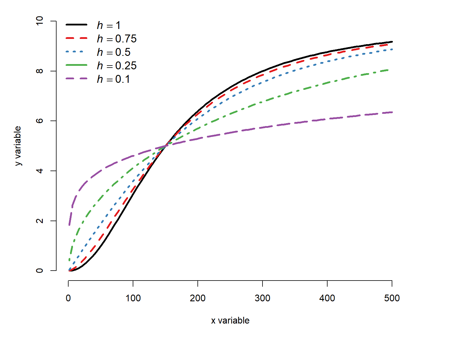

Figure 22.24: Five-parameter log-logistic curves with different \(h\) parameters, which control the symmetry of the curve about the midpoint \(g\). Values of \(h<1\) tend to flatten the curve, while values of \(h>1\) tend to make it steeper. The other parameters are constant at \(c=0\), \(d=10\), \(b=-8\), and \(g=5\).

The reason we had to adjust the midpoint to see the asymmetry wrought by \(h\) is that making the curve asymmetrical has the side effect of changing the slope at \(x=g\) (everywhere, really).

This is because at \(x=g\), \(\log{\left(x\right)}-\log{\left(x\right)}=0\), so the exponent equals \(b\left(0\right)=0\), so the exponential term \(e^{0}=1\), so:

\[f\left(x\right)=c+\frac{d-c}{\left(1+e^{b\left(\log{\left(x\right)}-\log{\left(x\right)}\right)}\right)^h}=c+\frac{d-c}{\left(1+1\right)^h}\]

When \(h=1\), this is halfway between the asymptotes. But when \(h<1\), \(2^h<2\), so \(f\left(g\right)>c+\left(d-c\right)/2\) (the function is greater than the halfway point). For our example where \(c=10\), \(d=10\), and \(b=-8\), decreasing \(h\) without adjusting \(g\) moves the point at which \(f\left(x\right)=5\) to the left:

x <- seq(1, 500, length=100)
B <- -2
C <- 0
D <- 10
G <- 150
H <- c(1, 0.75, 0.5, 0.25, 0.1)


cols <- c("black", "#e41a1c", "#377eb8", "#4daf4a","#984ea3")
par(mfrow=c(1,1), mar=c(5,5,1,4), 
    xpd=NA, bty="n")
plot(x, x, type="n", xlab="x variable",
     ylab="y variable", ylim=c(0, max(D)))
for(i in 1:length(H)){
    iy <- C+(D-C)/((1+exp(B*(log(x)-log(G))))^H[i])
    lines(x, iy, lwd=3, lty=i, col=cols[i])
}#i
legend("bottomright",
       legend=c(expression(italic(h)==1),
                expression(italic(h)==0.75),
                expression(italic(h)==0.5),
                expression(italic(h)==0.25),
                expression(italic(h)==0.1)),
       lty=1:3, lwd=3, col=cols,
       bty="n", cex=1.2)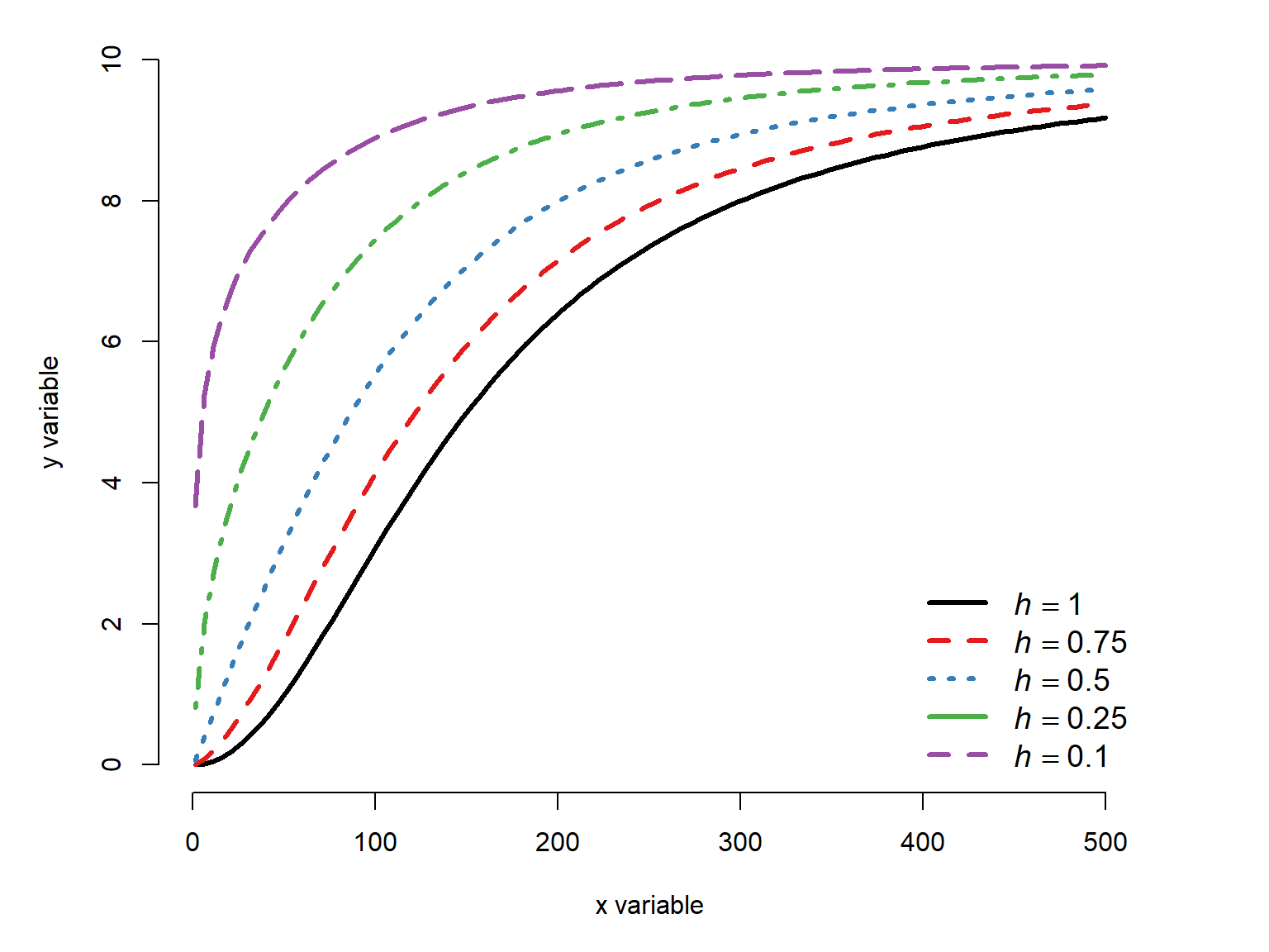

Figure 22.25: Five-parameter log-logistic curves with different \(h\) parameters, which control the symmetry of the curve about the midpoint \(g\), without adjusting \(g\). Values of \(h<1\) tend to flatten the curve, while values of \(h>1\) tend to make it steeper. The other parameters are constant at \(c=0\), \(d=10\), \(b=-8\), and \(g=5\).

Here is the effect of increasing \(h\) and adjusting \(g\) so that the midpoint remains at 5:

x <- seq(1, 500, length=100)
B <- -2
C <- 0
D <- 10
G <- 250
H <- c(1, 2, 10)


cols <- c("black", "#e41a1c", "#377eb8")
par(mfrow=c(1,1), mar=c(5,5,1,4), 
    xpd=NA, bty="n")
plot(x, x, type="n", xlab="x variable", 
     ylab="y variable", ylim=c(0, max(D)))
for(i in 1:length(H)){
    ig <- G / (2^(1/H[i])-1)^(1/B)
    iy <- C+(D-C)/((1+exp(B*(log(x)-log(ig))))^H[i])
    lines(x, iy, lwd=3, lty=i, col=cols[i])
}#i
legend("topleft",
       legend=c(expression(italic(h)==1),
                expression(italic(h)==5),
                expression(italic(h)==10)),
       lty=1:3, lwd=3, col=cols,
       bty="n", cex=1.2)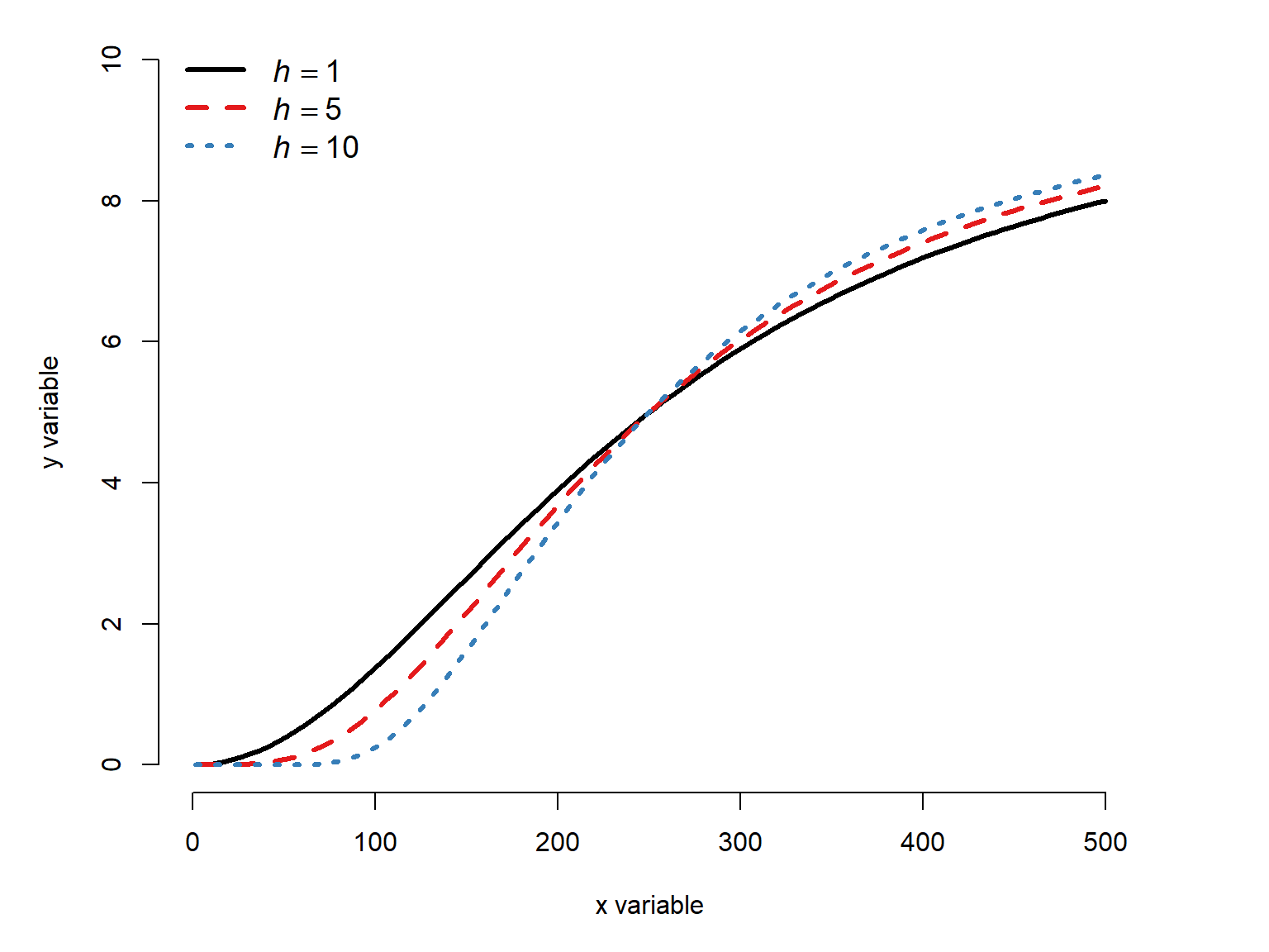

Figure 22.26: Five-parameter log-logistic curves with different \(h\) parameters, which control the symmetry of the curve about the midpoint \(g\). Values of \(h<1\) tend to flatten the curve, while values of \(h>1\) tend to make it steeper. The other parameters are constant at \(c=0\), \(d=10\), \(b=-8\), and \(g=5\).

Decreasing \(h\) has a much more drastic effect than increasing it.

22.2.5 Weibull curves

22.2.5.1 Derivation

The Weibull function describes a sigmoid curve between a lower and upper asymptote. So, it can behave much like a Gompertz or log-logistic curve, and is suitable in many of the same situations. Like the log-logistic group above, there are several versions of the Weibull function that with different numbers of parameters. Each additional parameter in the function allows another aspect of the curve to vary.

Like the log-logistic function, the Weibull function is derived from a probability distribution. The Weibull distribution is a continuous probability distribution often used for waiting times, similar to the gamma distribution. The cumulative distribution function (CDF) of the Weibull distribution for non-negative values is

\[F_{Weibull}\left(x\right)=1-e^{-\left(x/\lambda\right)^k}\]

where \(k\) and \(\lambda\) are the parameters of the distribution (shape and scale, respectively). We can take advantage of some exponent and logarithm rules to rewrite the Weibull CDF as a double exponential:

\[ \begin{aligned} F(x) &= 1-e^{-(x/\lambda)^k} && \qquad \text{Start with Weibull CDF}\\ F(x) &= 1-e^{-\left(\frac{x^k}{\lambda^k}\right)} && \qquad \text{Power of a quotient}\\ F(x) &= 1-e^{-e^{\log\left(\frac{x^k}{\lambda^k}\right)}} && \qquad \text{Definition of logarithm}\\ F(x) &= 1-e^{-e^{\log(x^k)-\log(\lambda^k)}} && \qquad \text{Logarithm of a quotient}\\ F(x) &= 1-e^{-e^{k\log(x)-k\log(\lambda)}} && \qquad \text{Power rule for logarithms}\\ F(x) &= 1-e^{-e^{k(\log(x)-\log(\lambda))}} && \qquad \text{Factor out } k \end{aligned} \]

This double exponential form of the Weibull CDF is sometimes called the “Type 2” Weibull function, including in the R package drc. The complement of the double exponential form of the Weibull CDF is the “Type 1” Weibull curve:

\[\text{Weibull curve}=e^{-e^{k\left(\log\left(x\right)-\log\left(\lambda\right)\right)}}\]

This version of the Weibull function has two parameters, and so it is called the two-parameter Weibull function. Like the two-parameter log-logistic, a three- and four-parameter version of the function can be defined by adding additional parameters to define an upper asymptote other than 1 (Section 22.2.5.3) and a lower asymptote other than 0 (Section 22.2.5.4). Unlike the log-logistic and the Gompertz functions, the Weibull function does not have a midpoint or inflection point as a parameter but it can be derived from parameters.

22.2.5.2 Two-parameter Weibull function

The two-parameter Weibull type 1 model is the basic Weibull function we derived in the previous section. We will use \(b\) instead of \(k\) for the shape parameter, and \(c\) instead of \(\lambda\) for the scale constant. It is given by

\[f\left(x\right)=e^{-e^{b\left(\log\left(x\right)-\log\left(c\right)\right)}}\] where \(b\) is the shape parameter and \(c\) is the scale parameter. This function has a lower asymptote at 0 and upper asymptote at 1. The figure below shows how the curve changes shape with different \(b\) parameters.

x <- seq(0.1, 10, length=100)
B <- -1*c(1, 2, 4, 8)
C <- 5

cols <- c("#e41a1c", "#377eb8", "#4daf4a","#984ea3")
par(mfrow=c(1,1), mar=c(5,5,1,4), 
    xpd=NA, bty="n")
plot(x, x, type="n", xlab="x variable",
     ylab="y variable", ylim=c(0, 1))
for(i in 1:length(B)){
    iy <- exp(-1*exp(B[i]*(log(x)-log(C))))
    points(x, iy, type="l", lwd=3,
           lty=i, col=cols[i])
    text(max(x)+0.2, max(iy),
         bquote(italic(b)==.(B[i])),
         adj=0, cex=1.2,
         col=cols[i])
}#i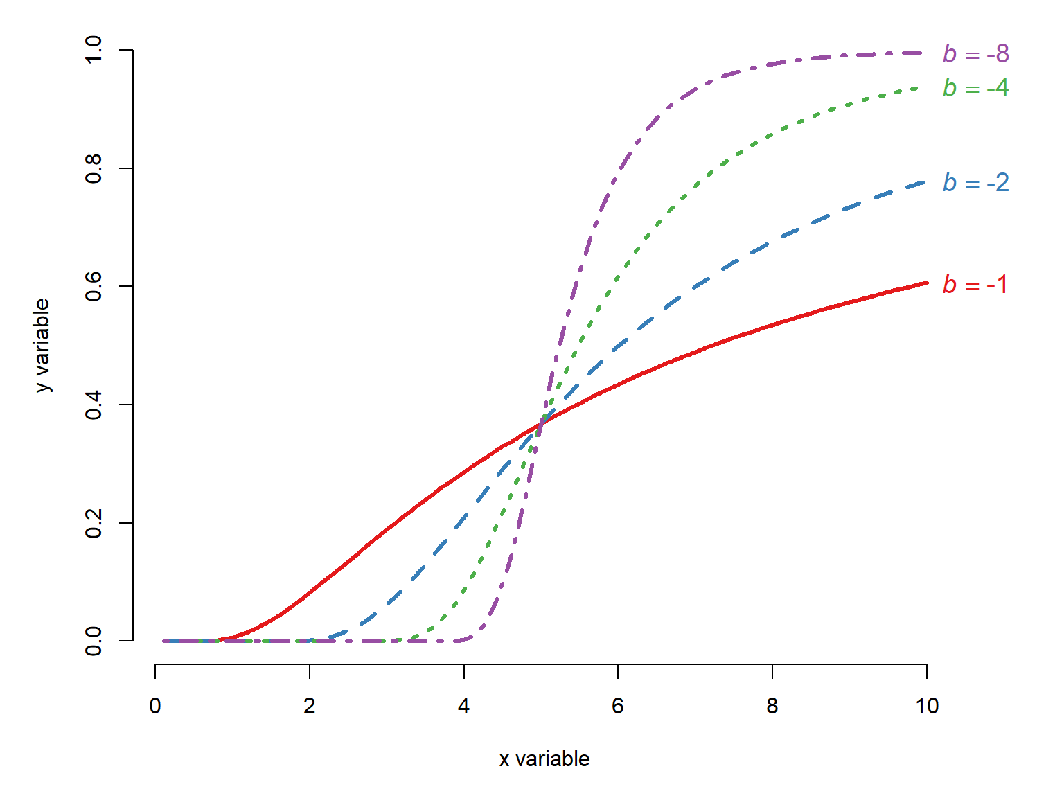

Figure 22.27: Two-parameter Weibull curves with different \(b\) parameters, which control the growth rate. Negative \(b\) of larger magnitude have steeper positive growth rates. The \(c\) parameter is fixed at 5.

Changing the \(c\) changes the function shape. It often has the effect of shifting the midpoint and the inflection point, but it represents neither of these directly.

x <- seq(0.1, 10, length=100)
B <- 5
C <- c(2, 4, 6, 8)

cols <- c("#e41a1c", "#377eb8", "#4daf4a", "#984ea3")
par(mfrow=c(1,1), mar=c(5,5,1,4), 
    xpd=NA, bty="n")
plot(x, x, type="n", xlab="x variable",
     ylab="y variable", ylim=c(0, 1))
for(i in 1:length(C)){
    iy <- exp(-1*exp(B*(log(x)-log(C[i]))))
    points(x, iy, type="l", lwd=3,
           lty=i, col=cols[i])
}#i
legend("topright",
       legend=c(
           expression(italic(c)==2),
           expression(italic(c)==4),
           expression(italic(c)==6),
           expression(italic(c)==8)),
       lty=1:length(C), lwd=3, col=cols,
       bty="n", cex=1.2)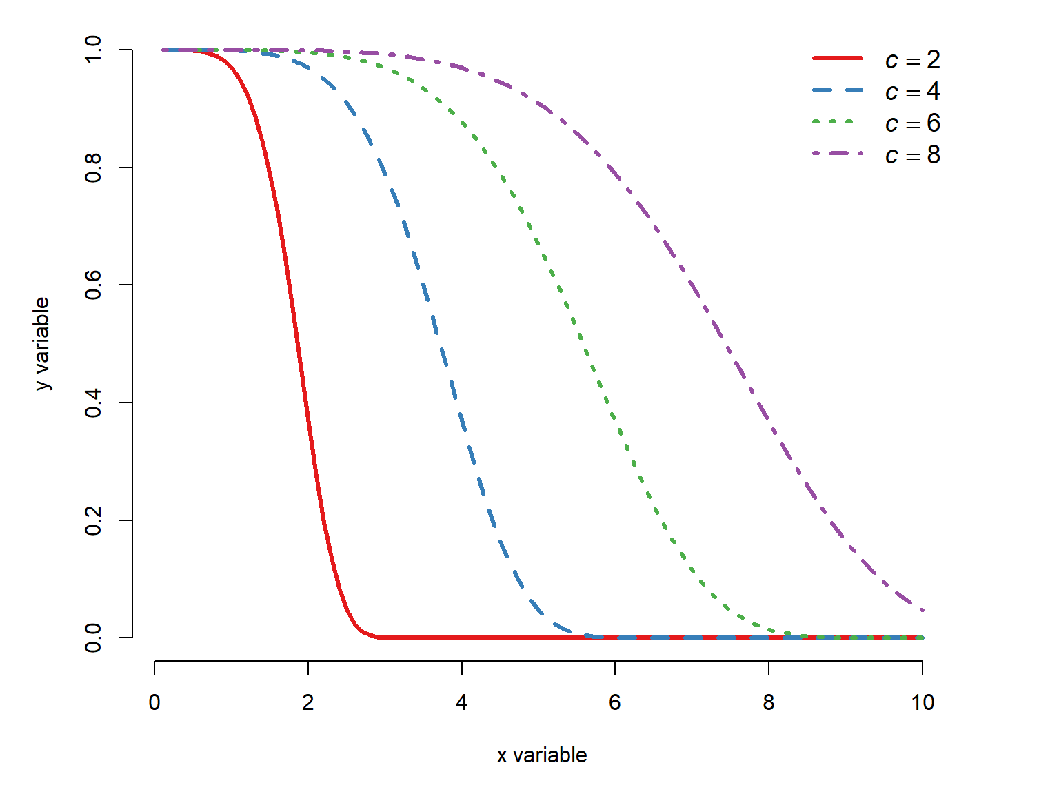

Figure 22.28: Two-parameter Weibull curves with different \(c\) parameters. The \(c\) parameter changes the function shape; it shifts the midpoint and the inflection point, but it represents neither of these directly. The \(b\) parameter is fixed at 5.

Figure 22.28 makes it seem that the scale parameter \(c\) shifts the function midpoint and the inflection point, but this isn’t actually true. The function midpoint calculated from both \(b\) and \(c\):

\[x_{mid}=ce^{\frac{\log{\left(-\log{\left(0.5\right)}\right)}}{b}}=ce^{\frac{\log{\left(\log{\left(2\right)}\right)}}{b}}\approx ce^{\frac{-0.3665}{b}}\]

the derivation of which is left as an exercise for the reader (I’ve always wanted to say that).

22.2.5.3 Three-parameter Weibull function

The three-parameter Weibull curve adds a parameter \(d\) to the two-parameter Weibull model to specify the upper asymptote:

\[f\left(x\right)=de^{-e^{b\left(\log{\left(x\right)}-\log{\left(c\right)}\right)}}\]

Varying the shape \(b\) or the scale \(c\) has the same effect as it does in the two-parameter Weibull (Figure 22.27, Figure 22.28), just with the upper asymptote shifted to \(d\).

22.2.5.4 Four-parameter Weibull function

Finally, the four-parameter Weibull curve adds one more parameter, \(a\), which can specify a lower asymptote other than 0:

\[f\left(x\right)=a+\left(d-a\right)e^{-e^{b\left(\log\left(x\right)-\log\left(c\right)\right)}}\] where \(b\) is the shape, \(c\) is the scale, \(d\) is the upper asymptote, and \(a\) is the lower asymptote.

When \(b\) is negative, the Weibull curve increases:

x <- seq(0.1, 10, length=100)
A <- 0
B <- -1*c(1, 2, 4, 8)
C <- 4
D <- 10


cols <- c("#e41a1c", "#377eb8", "#4daf4a","#984ea3")
par(mfrow=c(1,1), mar=c(5,5,1,4), 
    xpd=NA, bty="n")
plot(x, x, type="n", xlab="x variable",
     ylab="y variable", ylim=c(0, max(D)))
off <- c(0, 0, 0, 0.2)
for(i in 1:length(B)){
    iy <- A+(D-A)*exp(-1*exp(B[i]*(log(x)-log(C))))
    points(x, iy, type="l", lwd=3,
           lty=i, col=cols[i])
    text(max(x)+0.2, max(iy)+off[i],
         bquote(italic(b)==.(B[i])),
         adj=0, cex=1.2,
         col=cols[i])
}#i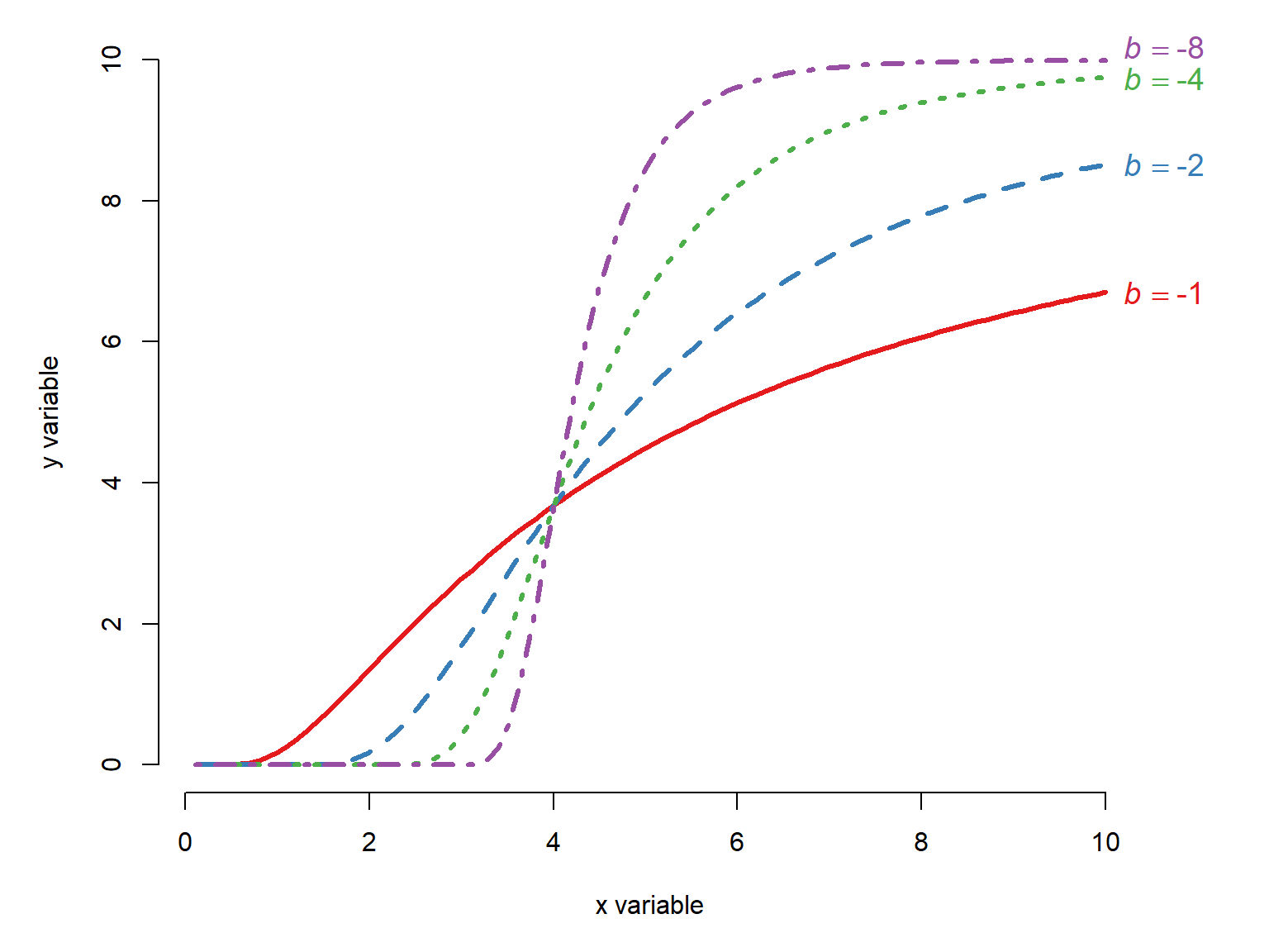

Figure 22.29: Four-parameter Weibull curves different \(b\) parameters, which control the growth rate. Negative \(b\) of larger magnitude have steeper positive growth rates. The other parameters are constant at \(a=0\), \(d=10\), and \(c=4\).

When \(b\) is positive, then the Weibull curve decreases:

x <- seq(0.1, 10, length=100)
A <- 0
B <- c(1, 2, 4, 8)
C <- 4
D <- 10


cols <- c("#e41a1c", "#377eb8", "#4daf4a","#984ea3")
par(mfrow=c(1,1), mar=c(5,5,1,4), 
    xpd=NA, bty="n")
plot(x, x, type="n", xlab="x variable",
     ylab="y variable", ylim=c(0, max(D)))
off <- c(0, 0, 0, 0.2)
for(i in 1:length(B)){
    iy <- A+(D-A)*exp(-1*exp(B[i]*(log(x)-log(C))))
    points(x, iy, type="l", lwd=3,
           lty=i, col=cols[i])
legend("topright",
       legend=c(
           expression(italic(b)==1),
           expression(italic(b)==2),
           expression(italic(b)==4),
           expression(italic(b)==8)),
       lty=1:length(B), lwd=3, col=cols,
       bty="n", cex=1.2)
}#i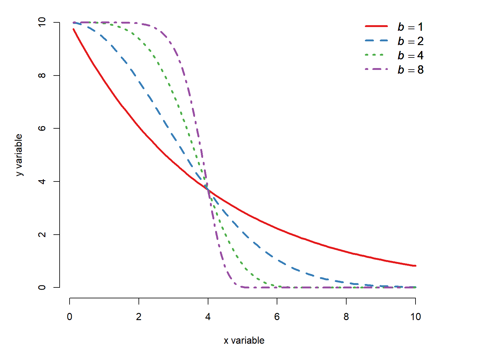

Figure 22.30: Four-parameter Weibull curves different \(b\) parameters, which control the growth rate. Positive \(b\) of larger magnitude have steeper negative growth rates. The other parameters are constant at \(a=0\), \(d=10\), and \(c=4\).

The \(c\) term changes the function shape, which often has the effect of shifting the midpoint to the left and right (even though \(c\) does not define the midpoint directly) or flattening or steepening the curve. Note that for some combinations of parameters, there may not be an inflection point visible in your data.

x <- seq(0.1, 10, length=100)
A <- 0
B <- -4
C <- c(2,4,6,8)
D <- 10


cols <- c("#e41a1c", "#377eb8", "#4daf4a","#984ea3")
par(mfrow=c(1,1), mar=c(5,5,1,4), 
    xpd=NA, bty="n")
plot(x, x, type="n", xlab="x variable",
     ylab="y variable", ylim=c(0, max(D)))
for(i in 1:length(C)){
    iy <- A+(D-A)*exp(-1*exp(B*(log(x)-log(C[i]))))
    points(x, iy, type="l", lwd=3,
           lty=i, col=cols[i])
}#i
legend("bottomright",
       legend=c(
           expression(italic(c)==2),
           expression(italic(c)==4),
           expression(italic(c)==6),
           expression(italic(c)==8)),
       lty=1:length(C), lwd=3, col=cols,
       bty="n", cex=1.2)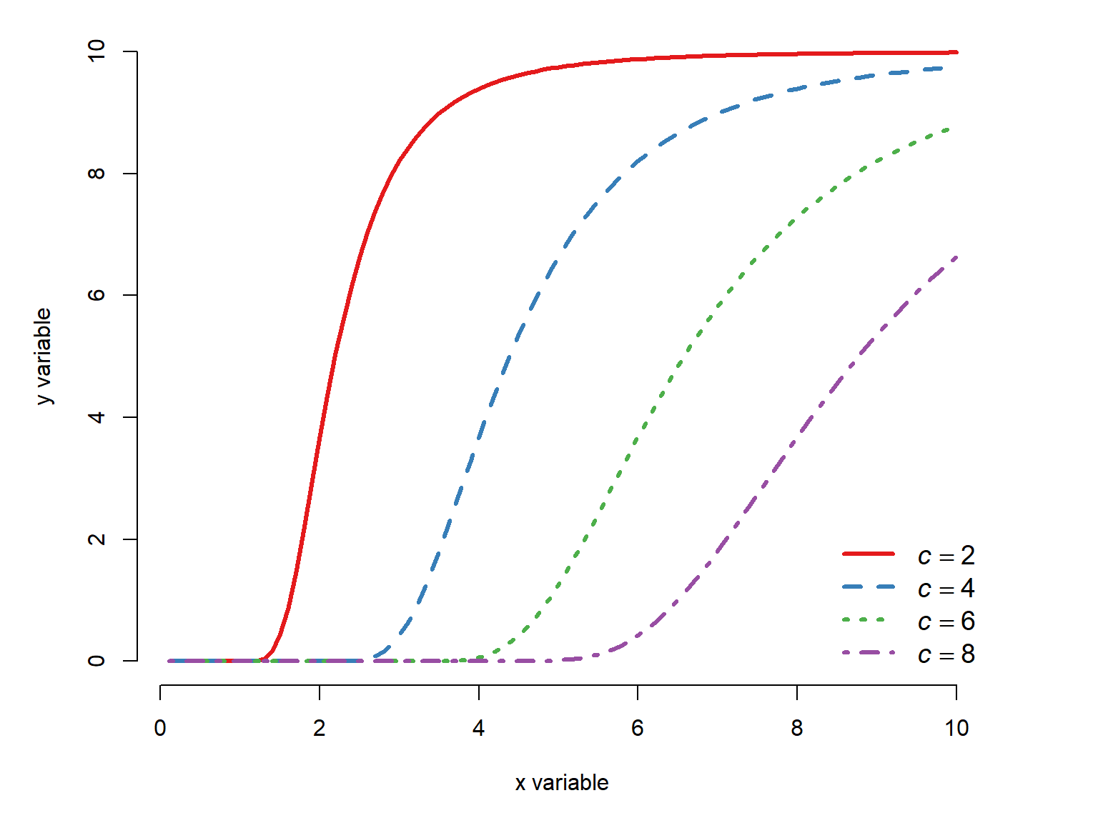

Figure 22.31: Four-parameter Weibull curves with different scale parameters \(c\), which change the shape of the curve. The other parameters are constant at \(a=0\), \(b=-4\), and \(d=10\).

22.2.6 Nonlinear functions summary

We have seen 5 types of nonlinear functions commonly used for biological data: the Michaelis-Menten, the Gompertz, the von Bertalanffy, the (log)-logistic, and the Weibull curves. Each of these can take on many shapes, and choosing which one to use to model your data requires both statistical know-how and, more importantly, biological judgement.

The functions that we explore can take on many shapes. So, the most important question is not, “Which curve looks the most like my scatterplot?” but rather “Which curve has parameters that make biological sense for my question?”. These curves are useful because they are defined in terms that describe biology quite well: minimum and maximum values, inflection points, midpoints, and growth rates.

Table 22.2: Comparison of parameters in common nonlinear growth models. “Derived” indicates that the characteristic point can be calculated from model parameters but is not itself a directly estimated parameter. A dash indicates that the characteristic is absent or not independently parameterized. *The Weibull type 1 curve has an interior inflection point only for appropriate values of its shape parameter.

Model	Lower asymptote	Upper asymptote	Midpoint	Inflection point	Growth rate / shape
Michaelis–Menten	\(0\) (fixed)	\(a\)	\(b\)	—	—
Gompertz (classic)	\(0\) (fixed)	\(a\)	Derived	\(\ln(b)/c\)	\(c\)
von Bertalanffy	\(0\) (fixed)	\(L_\infty\)	Derived	—	\(k\)
Log-logistic (2P)	\(0\) (fixed)	\(1\) (fixed)	\(g\)	Derived	\(b\) (slope)
Log-logistic (3P)	\(0\) (fixed)	\(d\)	\(g\)	Derived	\(b\) (slope)
Log-logistic (4P)	\(c\)	\(d\)	\(g\)	Derived	\(b\) (slope)
Log-logistic (5P)	\(c\)	\(d\)	\(g\)	Derived	\(b\) (slope), \(k\) (asymmetry)
Weibull type 1 (2P)	\(0\) (fixed)	\(1\) (fixed)	\(ce^{\log{\left(\log\left(2\right)\right)/b}}\)	Derived*	\(b\) (shape), \(c\) (scale)
Weibull type 1 (3P)	\(0\) (fixed)	\(d\)	\(ce^{\log{\left(\log\left(2\right)\right)/b}}\)	Derived*	\(b\) (shape), \(c\) (scale)
Weibull type 1 (4P)	\(a\)	\(d\)	\(ce^{\log{\left(\log\left(2\right)\right)/b}}\)	Derived*	\(b\) (shape), \(c\) (scale)

22.3 Nonlinear least squares with nls()

The basic nonlinear least squares (NLS) model has some parts in common with the basic linear regression model (LM). In the state-space GLM notation, we can see that the relationship between the observed \(y\) variable and the expected value \(\mu\) is the same as in the LM. However, the relationship between the expected value and the predictor variables is not the same.

\[y\sim \mathcal{Normal}\left(E\left(y\right),\sigma^2_{res}\right)\]

\[E\left(y\right)=\mathcal{f}\left(x\right)\]

where \(\mathcal{f}\left(x\right)\) is a nonlinear function of \(x\). In the NLS model, as with LM, the response variable \(y\) is drawn from a normal distribution with mean \(\mu\) and residual variance \(\sigma^2_{res}\). Unlike LM, in NLS the function for the expected value \(f\left(x\right)\) can be any number of functions.

The equations above show an important assumption of NLS: the errors are normally distributed with constant variance. If you need a another response distribution, then there are generalized nonlinear models that extend nonlinear models the way that GLM extends LM.

Unlike LM, where it is relatively straightforward to solve some linear algebra problems and get stable parameter estimates, in NLS the parameters must be approximated by searching the parameter space (i.e., set of possible values) for parameter values that minimize the sum of squared residuals. The methods for computing these estimates are extremely complicated and sensitive to starting inputs, and we won’t go into them here. Bolker (2008) gives an overview of some of these methods. The practical upshot for the average user is that starting values for the model must be supplied.

22.3.1 Fitting the model with self start functions

Let’s take a look at the NEON data. Download the individual measurement dataset and load it into R.

dx <- read.csv("data-neon-ind-meas.csv")

We will try a nonlinear model of ear length as a function of body length.

par(mar=c(5,5,1,1))
plot(dx$totalLength, dx$earLength,
     xlab="Total length (mm)",
     ylab="Ear length (mm)")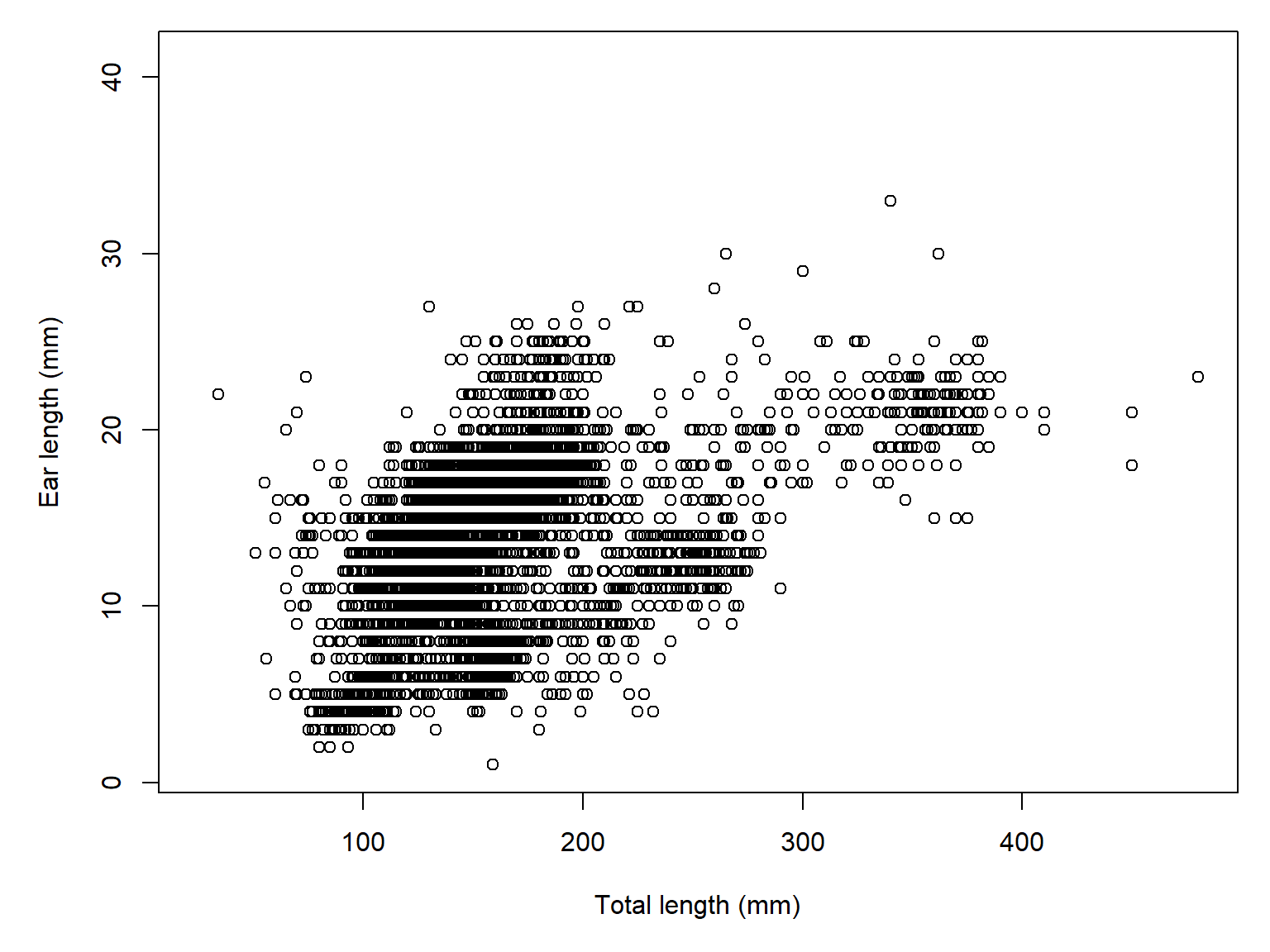

Figure 22.32: Ear length of small mammals appears to increase as a nonlinear function of total body length.

Models in nls() require starting values to prevent the algorithm from going too far afield. Finding appropriate values can be tricky. Fortunately, there are “self starting” models for many common functions (see ?selfStart for a list).

We will try a self-starting Michaelis-Menten function (SSmicmen) based not on any real biological basis, but rather the apparent shape of the curve.

mod1 <- nls(earLength~SSmicmen(totalLength,a,b), data=dx)
summary(mod1)

Formula: earLength ~ SSmicmen(totalLength, a, b)

Parameters:
  Estimate Std. Error t value Pr(>|t|)    
a  30.9866     0.7516   41.23   <2e-16 ***
b 184.2881     8.4823   21.73   <2e-16 ***
---
Signif. codes:  0 '***' 0.001 '**' 0.01 '*' 0.05 '.' 0.1 ' ' 1

Residual standard error: 3.752 on 6711 degrees of freedom

Number of iterations to convergence: 4 
Achieved convergence tolerance: 5.768e-06
  (142252 observations deleted due to missingness)

22.3.2 Fitting the model without self start functions

Sometimes we need to fit a model without a self starting function. This might be because we are fitting a model for which there is no self start function. Or, we need to feed an output to propagate to get confidence intervals. Either way, without a self starting function you will need to supply starting values for each parameter. This is usually done in a named list.

Below, we refit the ear length vs. body length relationship using the estimates from the self start model as starting values.

mod2 <- nls(earLength~(a*totalLength)/(b+totalLength),
            data=dx,
            start=list(a=30, b=180))
summary(mod2)

Formula: earLength ~ (a * totalLength)/(b + totalLength)

Parameters:
  Estimate Std. Error t value Pr(>|t|)    
a  30.9867     0.7516   41.23   <2e-16 ***
b 184.2890     8.4823   21.73   <2e-16 ***
---
Signif. codes:  0 '***' 0.001 '**' 0.01 '*' 0.05 '.' 0.1 ' ' 1

Residual standard error: 3.752 on 6711 degrees of freedom

Number of iterations to convergence: 3 
Achieved convergence tolerance: 7.171e-06
  (142252 observations deleted due to missingness)

If we don’t have a previous model fit to start with, we need to be clever. The best approach is to think about what the parameters really mean, and where they show up on the plot, and deduce from there. For example, for the ear length plot we might guess that the asymptote is no more than about 40 or 50. That is our starting guess for the \(a\) parameter. Then, we just need to eyeball where the curve reaches half of \(a\). Maybe 200 or so. That is our starting guess for the \(b\) parameter. Let’s try it.

mod3 <- nls(earLength~(a*totalLength)/(b+totalLength),
            data=dx,
            start=list(a=50, b=200))
summary(mod3)

Formula: earLength ~ (a * totalLength)/(b + totalLength)

Parameters:
  Estimate Std. Error t value Pr(>|t|)    
a  30.9858     0.7515   41.23   <2e-16 ***
b 184.2794     8.4819   21.73   <2e-16 ***
---
Signif. codes:  0 '***' 0.001 '**' 0.01 '*' 0.05 '.' 0.1 ' ' 1

Residual standard error: 3.752 on 6711 degrees of freedom

Number of iterations to convergence: 4 
Achieved convergence tolerance: 7.942e-06
  (142252 observations deleted due to missingness)

Even if your starting guesses are way off the algorithm should be able to find a fit. The rule here is “correct to an order of magnitude”.

22.3.3 Plotting a nonlinear curve

We can get a trendline in the usual way, by setting up a series of x values and calculating the predicted value at those values.

n <- 100
px <- seq(min(dx$totalLength, na.rm=TRUE),
          max(dx$totalLength, na.rm=TRUE), length=n)
prx <- data.frame(totalLength=px)
py <- predict(mod1, newdata=prx)


par(mar=c(5,5,1,1))
plot(dx$totalLength, dx$earLength,
     xlab="Total length (mm)",
     ylab="Ear length (mm)")
points(px, py, type="l", lwd=4, col="red")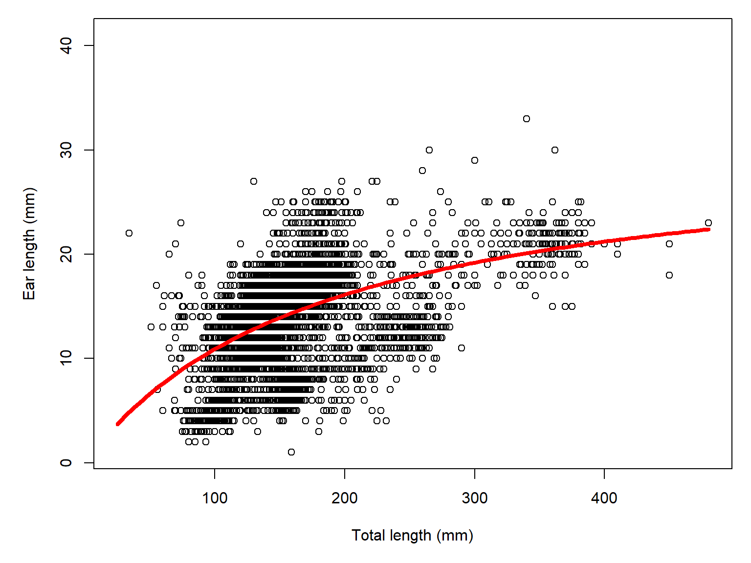

Figure 22.33: Ear length of small mammals appears to increase as a nonlinear function of total body length.

22.3.4 Confidence intervals for nonlinear models

Unlike lm() and glm(), there is no base option for generating confidence intervals on an nls() model. Instead, we need to use package propagate.

library(propagate)

Set up a series of \(x\) values and calculate a confidence interval. Note that if you use a self-start version of a model, you may get strange confidence intervals because propagate won’t be able to represent the model correctly. So, you may want to fit the selfStart version to get parameter estimates, then refit by specifying the model explicitly, using the parameter estimates from the selfStart() version as starting values. You can then use the estimates from the explicit version to generate confidence intervals.

n <- 10
px <- seq(min(dx$totalLength, na.rm=TRUE),
          max(dx$totalLength, na.rm=TRUE), length=n)
prx <- data.frame(totalLength=px)

# notice we use mod2, the explicitly coded model
# and not the selfStart version (which is mod1)
py <- predictNLS(mod2,
                 newdata=prx,
                 interval="confidence",
                 nsim=1e4) # default is 1e6; this is for speed

The predictNLS function actually estimates 3 versions of the confidence interval. The first two are by the Delta method, while the third is a Monte Carlo approximation. Usually the 3 estimates don’t disagree too much, and you usually can pick any of them. If one of them looks odd, go with one of the others.

# NOTE: this example uses R version 4.6.1 and
#       propagate version 1.2-0. The structure
#       of the predictNLS output is a bit 
#       different than previous versions of 
#       propagate (e.g., 1.0-7).
# first order delta approximation
prx$mn <- py$summary[,1] # mean.1
prx$lo <- py$summary[,5] # 2.5% (first one)
prx$up <- py$summary[,6] # 97.5% (first one)

par(mar=c(5,5,1,1))
plot(dx$totalLength, dx$earLength,
     xlab="Total length (mm)",
     ylab="Ear length (mm)")
points(px, prx$mn, type="l", lwd=3, col="red")
points(px, prx$lo, type="l", lwd=2, col="red", lty=2)
points(px, prx$up, type="l", lwd=2, col="red", lty=2)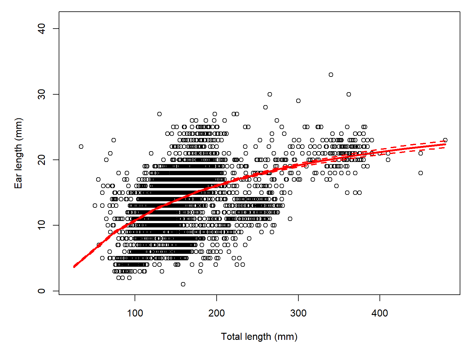

Figure 22.34: Ear length of small mammals appears to increase as a nonlinear function of total body length. Thick line shows predicted value and dashed lines show 95% confidence interval.

22.3.5 Factors and interactions in nonlinear models

Unlike lm() and glm(), adding factors and interactions in nls() takes a bit of coding. The trick is to write the model function explicitly with group-specific parameters, and include a multiplier to multiply those parameters by 0 for observations where they aren’t needed. Let’s fit a different curve for ear length in two families, Cricetidae and Muridae. Download the taxonomic dataset and use it to filter the individual measurements dataset.

tax <- read.csv("data-neon-taxa.csv")

use.vars <- c("abb", "totalLength", "earLength")
dx2 <- dx[complete.cases(dx[,use.vars]),]


dx2$family <- tax$family[match(dx2$abb,tax$abb)]

# cricetid species
cri <- tax$abb[which(tax$family=="Cricetidae")]
# murid species
mur <- tax$abb[which(tax$family=="Muridae")]

dx2 <- dx2[which(dx2$abb %in% c(cri, mur)),]


# colors and shapes
cols <- c("#4F94CD4D", "tomato3")
names(cols) <- c("Cricetidae", "Muridae" )
pchs <- c(0, 1)
names(pchs) <- names(cols)
dx2$col <- cols[dx2$family]
dx2$pch <- pchs[dx2$family]

par(mar=c(5,5,1,1))
plot(dx2$totalLength, dx2$earLength,
     xlab="Total length (mm)",
     ylab="Ear length (mm)",
     col=dx2$col, pch=dx2$pch)
legend("topleft", legend=names(cols),
       pch=pchs, col=cols,
       cex=1.2,bty="n")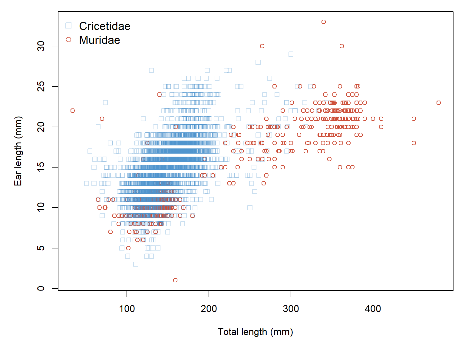

Figure 22.35: Ear length of Cricetid and Murid rodents appears to increase as a nonlinear function of total body length.

Add an indicator variable for each group, for each level of our factor. The value is 1 for observations in the group, and 0 otherwise.

dx2$cr <- ifelse(dx2$family=="Cricetidae", 1, 0)
dx2$mu <- ifelse(dx2$family=="Muridae", 1, 0)

Now construct the model.

mod4 <- nls(earLength~cr*((a.cr*totalLength)/(b.cr+totalLength))+
                      mu*((a.mu*totalLength)/(b.mu+totalLength)),
            data=dx2,
            start=list(a.cr=50, b.cr=180, a.mu=20, b.mu=180))
summary(mod4)

Formula: earLength ~ cr * ((a.cr * totalLength)/(b.cr + totalLength)) + 
    mu * ((a.mu * totalLength)/(b.mu + totalLength))

Parameters:
     Estimate Std. Error t value Pr(>|t|)    
a.cr   50.438      1.967   25.64   <2e-16 ***
b.cr  344.067     19.606   17.55   <2e-16 ***
a.mu   49.646      2.198   22.59   <2e-16 ***
b.mu  487.649     32.800   14.87   <2e-16 ***
---
Signif. codes:  0 '***' 0.001 '**' 0.01 '*' 0.05 '.' 0.1 ' ' 1

Residual standard error: 2.404 on 5629 degrees of freedom

Number of iterations to convergence: 4 
Achieved convergence tolerance: 7.632e-06

Now make the trendlines. Remember that the data frame you pass to the predict call has to have every variable that went into the analysis…even the indicators variables like cr and mu.

px1 <- seq(min(dx2$totalLength[dx2$family=="Cricetidae"]),
           max(dx2$totalLength[dx2$family=="Cricetidae"]),
           length=100)
px2 <- seq(min(dx2$totalLength[dx2$family=="Muridae"]),
           max(dx2$totalLength[dx2$family=="Muridae"]),
           length=100)
py1 <- predict(mod4,
               newdata=data.frame(totalLength=px1,
                                  cr=1, mu=0))
py2 <- predict(mod4, newdata=data.frame(totalLength=px2,
                                        cr=0, mu=1))

par(mar=c(5,5,1,1))
plot(dx2$totalLength, dx2$earLength,
     xlab="Total length (mm)",
     ylab="Ear length (mm)",
     col=dx2$col, pch=dx2$pch)
points(px1, py1, type="l", lwd=4, col="steelblue4")
points(px2, py2, type="l", lwd=4, col=cols[2], lty=2)
legend("topleft", legend=names(cols),
       pch=pchs, col=c("steelblue4", cols[2]), lwd=4, lty=c(1,2),
       cex=1.2,bty="n")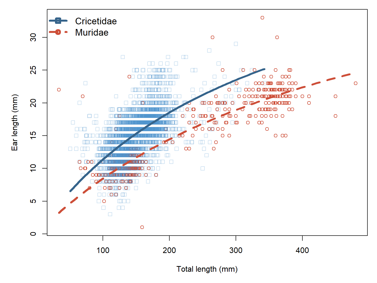

Figure 22.36: Ear length of Cricetid and Murid rodents appears to increase as a nonlinear function of total body length. Thick lines shows predicted value and dashed lines show 95% confidence interval.

22.3.6 Significance and nonsignificance in nonlinear models

The p-values in an nls() summary test whether each estimated parameter differs from zero, using an approximation based on the parameter’s standard error. These tests are not necessarily meaningful for nonlinear models, especially when parameters have biological constraints or zero represents a degenerate model. For example, a nonsignificant asymptote term \(a\) in a Michaelis-Menten model or log-logistic model (\(d\)) may be mathematically valid, but biologically nonsensical. Instead of relying on p-values, focus primarily on parameter estimates, their confidence intervals, and how well the model describes the observed relationship.

22.4 Dose-response curves with drc

A dose response curve describes the change in a biological system following a quantitative perturbation. Most dose response models are nonlinear because of the dynamics of the systems they describe. Mechanistically, there is often a rate that scales with the current concentration of a compound, or some other aspect of the system. In other words, the dynamics of the system are described by a kind of differential equation. The state of the system is thus described by solutions to those equations.

One of the most popular packages for fitting dose response models is package drc (Ritz et al. (2015)). This package provides functions for fitting all of the nonlinear functions described in this module, as well others we haven’t seen. You can see the functions available in drc with the function drc::getMeanFunctions().

I simulated some dose-response data for us to practice with. Download the simulated dose-response data. If you want to see how the data were simulated, unfold the code block below:

# random number seed
set.seed(123)

# experimental parameters
## concentrations tested
concs <- c(0, 10, 25, 50, 100, 200, 300, 400, 500)
## species tested
spp <- 1:2
## replicates per species * concentration combination
repl <- 1:5
## make data frame
dx <- expand.grid(conc=concs, species=spp, repl=repl)

# "true" model parameters
C <- 0
D <- 1
B <- c(-2, -4)
G <- c(80, 200)

# expected p(mortality)
# four-parameter log-logistic model
dx$ey <- C+(D-C)/(1+exp(B[dx$species]*(log(dx$conc)-log(G[dx$species]))))

# assign colors and symbols
pchs <- c(15, 16)
cols <- rainbow(length(B))
dx$pch <- pchs[dx$species]
dx$col <- cols[dx$species]

# simulate mortality within each trial
# and calculate percent mortality
dx$size <- 50
dx$mort <- rbinom(nrow(dx), size=dx$size, prob=dx$ey)
dx$pmort <- 100*dx$mort / dx$size

# export
out <- dx[,c("conc", "species", "repl", "size", "pmort")]
out$species <- LETTERS[out$species]
write.csv(out, "data-sim-dose-response.csv", row.names=FALSE)

Import the data:

dx <- read.csv("data-sim-dose-response.csv")

This dataset contains simulated data from a toxic exposure experiment where two species of, say, midges were exposed to different concentrations of an experimental pesticide. Midge eggs were placed in jars, 50 per jar, with 10 replicates (variable repl) per species \(\times\) concentration combination. The researchers recorded how many larvae out of 50 died in each jar and recorded this as percent mortality (variable pmort). Pesticide concentration is variable conc, and size is the number of larvae per jar.

Let’s add some symbology to the dataset so we can visualize the data.

# assign colors and symbols
pchs <- c(15, 16)
cols <- c("red", "blue")
species <- sort(unique(dx$species))
names(pchs) <- species
names(cols) <- species
dx$pch <- pchs[dx$species]
dx$col <- cols[dx$species]

Now make a plot with different colors and symbols for each species.

par(mfrow=c(1,1), mar=c(5,5,1,1), xpd=NA, bty="n")
plot(dx$conc, dx$pmort, col=dx$col, pch=dx$pch,
     xlab=expression(Pesticide~concentration~(mu*g/L)),
     ylab="Mortality (%)")
legend("bottomright", legend=species,
       pch=pchs, col=cols, cex=1.2, bty="n")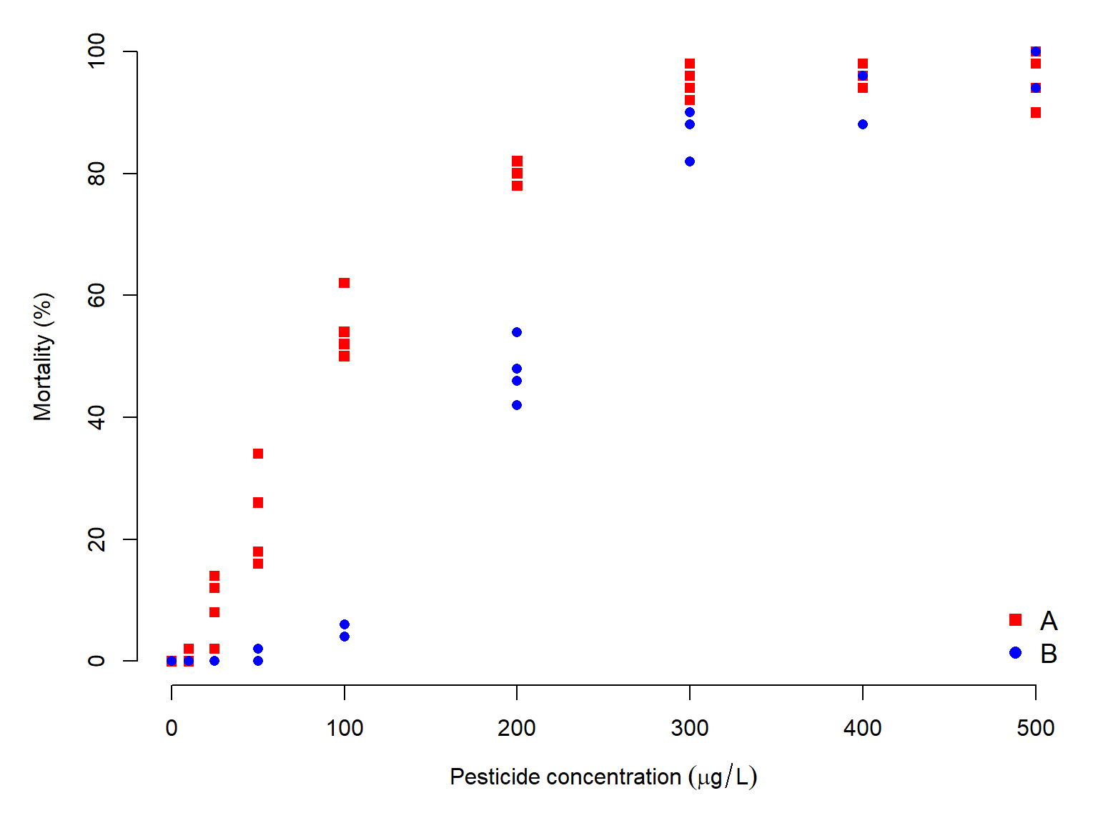

Figure 22.37: Data from a simulated toxic exposure trial where larval midges were exposed to different concentrations of an experimental pesticide. The percentage of larvae that die increases with concentration for both species A and species B, with mortality increasing faster in species A. Both species exhibit nearly 100% mortality above 300 μg/L.

It looks like mortality increases with concentration, which makes sense. It also looks like the two species A and B respond differently, with mortality increasing faster in species A than in species B. Let’s test this observation by fitting some curves.

22.4.1 Single groups

We can use drc to fit the data to one species or to multiple species. Let’s fit some curves to species A first. Filter the dataset to just that species. Then we will fit several models and compare them using AIC.

library(drc)

The percentage mortality variable represents a proportion, whose denominator is the size column (number of midges per trial). Recall from Section 21.2 that proportions are analyzed using the binomial distribution and a “weights” argument that defines the denominator of each proportion. We will have to specify that in drm() just as we do in glm(). Each call to drm() also takes the argument fct which specifies which model to fit. See getMeanFunctions() to see a list of available models.

Note: Fitting these models may generate warnings such as NaNs produced. These occur when the numerical optimization algorithm explores parameter values for which the model is mathematically undefined (e.g., a negative midpoint parameter). Such warnings do not necessarily indicate a problem with the final fitted model. If the model converges successfully, its parameter estimates are biologically reasonable, and its fitted curve adequately describes the data, these warnings can generally be disregarded.

# filter to species A only
da <- subset(dx, dx$species=="A")

# convert percent to proportion
da$pmort.y <- da$pmort / 100

mod01 <- drm(pmort.y~conc, data=da, fct=LL.2(),
             type="binomial", weights=size)
mod02 <- drm(pmort.y~conc, data=da, fct=LL.3(),
             type="binomial", weights=size)
mod03 <- drm(pmort.y~conc, data=da, fct=LL.4(),
             type="binomial", weights=size)
mod04 <- drm(pmort.y~conc, data=da, fct=W1.2(),
             type="binomial", weights=size)
mod05 <- drm(pmort.y~conc, data=da, fct=W1.3(),
             type="binomial", weights=size)
mod06 <- drm(pmort.y~conc, data=da, fct=W1.4(),
             type="binomial", weights=size)

Now check the model coefficients:

# put in a list
mod.list <- list(mod01, mod02, mod03, mod04, mod05, mod06)
names(mod.list) <- paste0("mod",
                          formatC(1:6, width=2, flag="0"))
# inspect coefficients
lapply(mod.list, coef)

$mod01
b:(Intercept) e:(Intercept) 
    -2.001158     87.201257 

$mod02
b:(Intercept) d:(Intercept) e:(Intercept) 
    -1.967928      1.005026     88.215297 

$mod03
b:(Intercept) c:(Intercept) d:(Intercept) e:(Intercept) 
 -1.956583586  -0.001248771   1.005742038  88.093970709 

$mod04
b:(Intercept) e:(Intercept) 
    -1.267799     53.926659 

$mod05
b:(Intercept) d:(Intercept) e:(Intercept) 
   -0.9806101     1.1225292    65.6721373 

$mod06
b:(Intercept) c:(Intercept) d:(Intercept) e:(Intercept) 
 -1.075057267   0.003799968   1.092910824  64.958680664 

The fitted coefficients look pretty sensible. We should also check convergence.

sapply(mod.list, function(x){x$fit$convergence})

mod01 mod02 mod03 mod04 mod05 mod06 
 TRUE  TRUE  TRUE  TRUE  TRUE  TRUE 

Before we do any model comparison, we need to check the predicted values of each model. Just because a drm model is converged and has sensible-looking parameters, does not mean it actually fits the data very well. Sometimes these models can get goofy fits that should disqualify them.

par(mfrow=c(3,2))
for(i in 1:length(mod.list)){
    plot(mod.list[[i]],
         main=names(mod.list)[i])
}

Figure 22.38: Quick figures showing 6 nonlinear models fitted to data from a simulated toxic exposure trial. The data represent an experiment where larval midges were exposed to different concentrations of an experimental pesticide. The percentage of larvae that die increases with concentration.

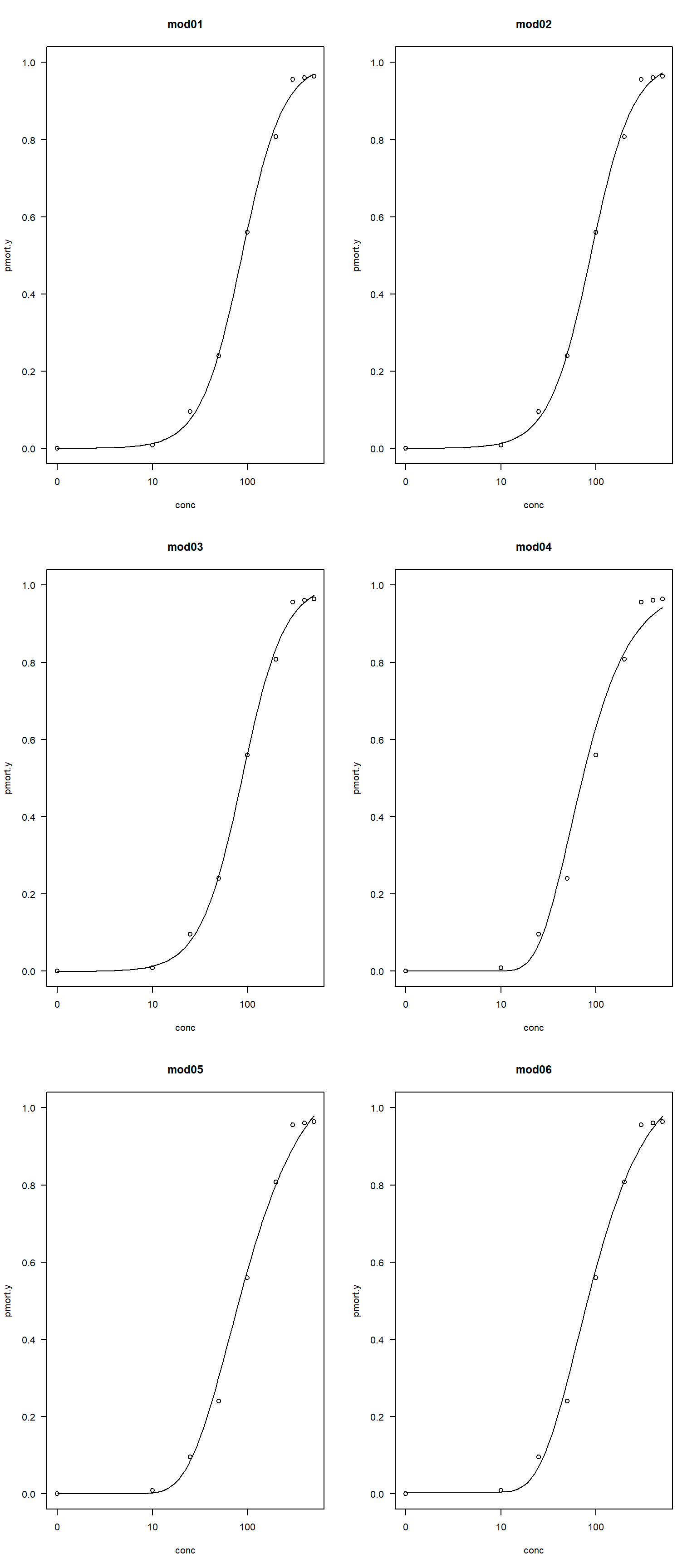
All of the figures look fine, so let’s compare all 6 models.

# get model AIC
aicdf <- data.frame(mod=names(mod.list),
                    aic=sapply(mod.list, AIC))

# calculate delta AIC
aicdf$delta <- aicdf$aic-min(aicdf$aic)

# calculate relative likelihood
aicdf$rel <- exp(-0.5*aicdf$delta)

# normalize to convert to aic weight
aicdf$wt <- aicdf$rel/sum(aicdf$rel)

# order by delta
aicdf <- aicdf[order(aicdf$delta),]
# round
aicdf[,-1] <- round(aicdf[,-1], 2)
aicdf

        mod    aic delta  rel   wt
mod01 mod01 163.65  0.00 1.00 0.64
mod02 mod02 165.51  1.85 0.40 0.26
mod03 mod03 167.38  3.73 0.16 0.10
mod05 mod05 180.27 16.62 0.00 0.00
mod06 mod06 180.35 16.69 0.00 0.00
mod04 mod04 205.02 41.37 0.00 0.00

The best supported model was model 1, the two-parameter log-logistic, with an AIC weight of 0.64. This means that the probability that this model is the best supported model among these 6 candidate models is 0.64. Model 2, the three-parameter log-logistic, has a \(\Delta AIC\) less than 2, so we cannot rule it out. The two-parameter log-logistic being the best-fitting model makes sense. Figure 22.38 shows that the mortality rates span the range from 0 to 1, so the extra terms in the three- and four-parameter log-logistic models that specify other asymptotes are not needed.

22.4.2 Multiple groups

We can also fit dose response curves to multiple groups at once. Let’s analyze the full dose-response dataset and compare the curves for species A and B.

dx$pmort.y <- dx$pmort / 100

mod07 <- drm(pmort.y~conc, curveid=species, data=dx, fct=LL.2(),
             type="binomial", weights=size)
mod08 <- drm(pmort.y~conc, curveid=species, data=dx, fct=LL.3(),
             type="binomial", weights=size)
mod09 <- drm(pmort.y~conc, curveid=species, data=dx, fct=LL.4(),
             type="binomial", weights=size)
mod10 <- drm(pmort.y~conc, curveid=species, data=dx, fct=W1.2(),
             type="binomial", weights=size)
mod11 <- drm(pmort.y~conc, curveid=species, data=dx, fct=W1.3(),
             type="binomial", weights=size)
mod12 <- drm(pmort.y~conc, curveid=species, data=dx, fct=W1.4(),
             type="binomial", weights=size)

Once again, check for convergence.

# put in a list
mod.list2 <- list(mod07, mod08, mod09, mod10, mod11, mod12)
names(mod.list2) <- paste0("mod",
                          formatC(7:12, width=2, flag="0"))
# inspect coefficients
lapply(mod.list2, coef)

$mod07
       b:A        b:B        e:A        e:B 
 -2.001158  -4.157096  87.202123 199.738435 

$mod08
        b:A         b:B         d:A         d:B         e:A         e:B 
 -1.9675589  -4.2767121   1.0050434   0.9932908  88.2303331 198.3661663 

$mod09
          b:A           b:B           c:A           c:B           d:A 
-1.945466e+00 -4.286436e+00 -2.382218e-03 -1.773330e-06  1.006493e+00 
          d:B           e:A           e:B 
 9.927768e-01  8.796731e+01  1.982687e+02 

$mod10
       b:A        b:B        e:A        e:B 
 -1.267859  -2.319653  53.929612 149.475972 

$mod11
        b:A         b:B         d:A         d:B         e:A         e:B 
 -0.9806254  -1.8353159   1.1225321   1.1242760  65.6723157 168.1432049 

$mod12
          b:A           b:B           c:A           c:B           d:A 
 -1.074855053  -2.377770958   0.003776190   0.002104492   1.092961978 
          d:B           e:A           e:B 
  1.053349887  64.958256592 166.473270107 

And check the plots for reasonableness.

par(mfrow=c(3,2))
for(i in 1:length(mod.list2)){
    plot(mod.list2[[i]],
         main=names(mod.list2)[i],
         legendPos=c(5, 1))
}

Figure 22.39: Quick figures showing 6 nonlinear models fitted to data from a simulated toxic exposure trial with two species of midge. The data represent an experiment where larval midges were exposed to different concentrations of an experimental pesticide. The percentage of larvae that die increases with concentration.

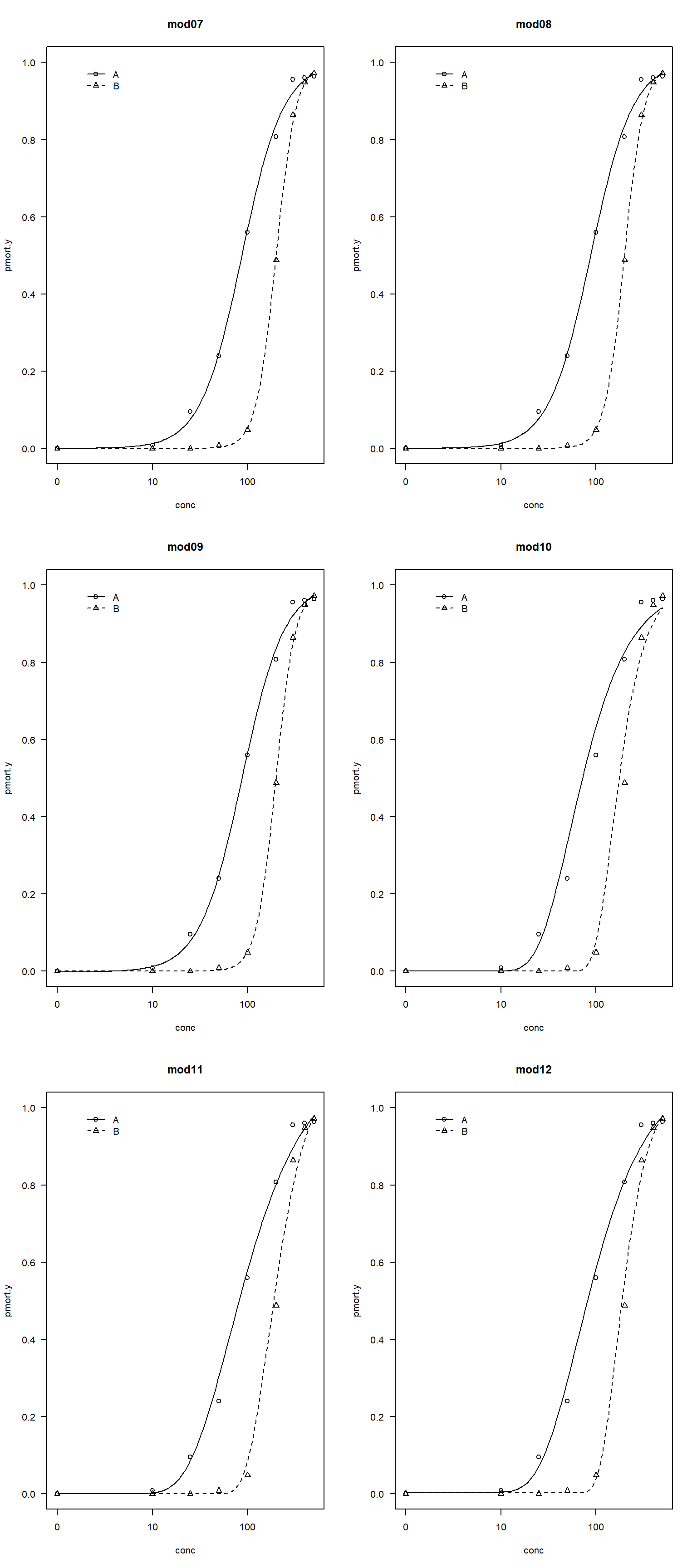
All of the fitted curves look okay. Let’s compare models using AIC.

# get model AIC
aicdf2 <- data.frame(mod=names(mod.list2),
                    aic=sapply(mod.list2, AIC))

# calculate delta AIC
aicdf2$delta <- aicdf2$aic-min(aicdf2$aic)

# calculate relative likelihood
aicdf2$rel <- exp(-0.5*aicdf2$delta)

# normalize to convert to aic weight
aicdf2$wt <- aicdf2$rel/sum(aicdf2$rel)

# order by delta
aicdf2 <- aicdf2[order(aicdf2$delta),]
# round
aicdf2[,-1] <- round(aicdf2[,-1])
aicdf2

        mod aic delta rel wt
mod07 mod07 272     0   1  1
mod08 mod08 276     4   0  0
mod09 mod09 280     7   0  0
mod12 mod12 305    33   0  0
mod11 mod11 322    50   0  0
mod10 mod10 371    98   0  0

In this case, model 7 (the two-parameter log-logistic) is by far the best supported. We will interpret that model.

First, inspect the coefficients. The fitted parameters are very close to the truth.

summary(mod07)

Model fitted: Log-logistic (ED50 as parameter) with lower limit at 0 and upper limit at 1 (2 parms)

Parameter estimates:

      Estimate Std. Error t-value   p-value    
b:A  -2.001158   0.081684 -24.499 < 2.2e-16 ***
b:B  -4.157096   0.216370 -19.213 < 2.2e-16 ***
e:A  87.202123   3.151717  27.668 < 2.2e-16 ***
e:B 199.738435   4.494227  44.443 < 2.2e-16 ***
---
Signif. codes:  0 '***' 0.001 '**' 0.01 '*' 0.05 '.' 0.1 ' ' 1

Because the ED50, or dose expected to cause 50% mortality, is a parameter in the log-logistic model (e), we don’t need to calculate it. However, we use the ED() function to get the estimates and their 95% confidence intervals.

ED(mod07, 50, interval="delta")

Estimated effective doses

       Estimate Std. Error    Lower    Upper
e:A:50  87.2021     3.1517  81.0249  93.3794
e:B:50 199.7384     4.4942 190.9299 208.5470

Note that ED() defaults to relative response levels. Thus, ED50 represents the dose producing a response halfway between the fitted lower and upper asymptotes. For LL.2(), those asymptotes are fixed at 0 and 1, so ED50 is also the dose corresponding to 50% mortality. If you fit a model where the asymptotes are not 0 and 1, you need to add the argument type="absolute" and set respLev=0.5 instead of 50. Otherwise, the ED50 won’t be a true ED50; it will be an ED-“whatever value is halfway between the upper and lower asymptotes”.

ED(mod07, 0.5, interval="delta", type="absolute")

Estimated effective doses

        Estimate Std. Error    Lower    Upper
e:A:0.5  87.2021     3.1517  81.0249  93.3794
e:B:0.5 199.7384     4.4942 190.9299 208.5470

One caveat: if 0.5 lies outside the range of responses predicted by the fitted model, then an absolute ED50 doesn’t exist, and ED() may return NaN or another non-finite result.

For comparing ED50 (or any parameter) between species A and B, you can use a Wald test of the difference between parameter estimates. Package drc has function compParm() that does this:

compParm(mod07, "e", operator="-")

Comparison of parameter 'e' 

     Estimate Std. Error t-value   p-value    
A-B -112.5363     5.4892 -20.501 < 2.2e-16 ***
---
Signif. codes:  0 '***' 0.001 '**' 0.01 '*' 0.05 '.' 0.1 ' ' 1

Alternatively, you can compare effective doses directly:

EDcomp(mod07, c(50, 50), interval = "delta")

Estimated ratios of effect doses

          Estimate   Lower   Upper
A/B:50/50  0.43658 0.40015 0.47301

or if you have asymptotes other than 0 and 1:

EDcomp(mod07, c(0.5, 0.5), interval = "delta", type="absolute")

Estimated ratios of effect doses

            Estimate   Lower   Upper
A/B:0.5/0.5  0.43658 0.40015 0.47301

22.5 Generalized additive models (GAM)

Coming soon!

22.6 Generalized nonlinear models (GNM)

Coming soon!

22.7 Regression trees for nonlinear patterns

Coming soon!

Bolker BM. 2008. Ecological models and data in R. Princeton, New Jersey, USA: Princeton University Press.

Green NS, Wildhaber ML, Albers JL, Pettit TW, Hooper MJ. 2020. Efficient mammal biodiversity surveys for ecological restoration monitoring. Integrated Environmental Assessment and Management.

Kunz BK, Waddle JH, Green NS. 2019. Amphibian monitoring in hardwood forests: Optimizing methods for contaminant-based compensatory restorations. Integrated environmental assessment and management.

Ritz C, Baty F, Streibig JC, Gerhard D. 2015. Dose-response analysis using R. PLoS ONE 10(12):e0146021. https://doi.org/10.1371/journal.pone.0146021