dat <- read.csv("data-neon-ind-meas.csv")
met <- read.csv("data-neon-metadata-site.csv")23 Random effects and mixed models
23.1 Introduction
So far, the linear models (LMs) and generalized linear models (GLMs) we have studied have included two components:
- A systematic component (or deterministic component), which describes how the expected value of the response variable depends on the predictor variables.
- A stochastic component, which describes random variation in the response variable around its expected value.
For example, consider a linear regression describing the relationship between body mass and metabolic rate:
\[ Y_i=\beta_0+\beta_1X_i+\varepsilon_i \]
The systematic component is \(\beta_0+\beta_1X_i\), which describes the expected metabolic rate for an animal of a given body mass. The stochastic component is \(\varepsilon_i\), which describes the variation in metabolic rate that the systematic component does not explain. In an ordinary linear model, we generally assume that the residuals are independent and identically distributed, with mean zero and variance \(\sigma^2_{res}\). Another way to state that i.i.d. assumption is that the residual variation is unstructured.
But what if some of that unexplained variation has an identifiable structure?
Suppose our animals were measured in several different laboratories. Measurements from the same laboratory might be more similar to each other than measurements from different laboratories, perhaps because of differences in equipment, experimental protocols, or environmental conditions. This inter-laboratory variation has a structure, but it is not a structure that we as researchers are interested in. We want to account for it, certainly, but we are not interested in these laboratories themselves as experimental units.
Our original linear model does not explicitly account for this source of variation. We could add laboratory as a categorical predictor, as we did in analysis of covariance (ANCOVA). If we assume that the metabolic rate measurements were differently calibrated in each laboratory, that model would look like:
\[ Y_i=\beta_0+\beta_{1,lab_i}+\beta_2X_i+\varepsilon_i \]
This model adds a term \(\beta_{1,lab}\) that captures the lab-specific effect. This term functions as an extra intercept, so we could also have written:
$$ Y_i=_{0,lab_i}+_1X_i+_i
$$
Where the lab determines the intercept directly. In either case, we are fitting the effect of lab as we do any other model parameter, such as the slope for body mass. The fitted lab-specific intercepts describe differences among the particular laboratories that made the measurements, potentially reflecting differences in equipment, experimental conditions, or other factors.
It is worth asking the question: “Do we care about the differences between Laboratories A, B, and C specifically, or do we primarily want to account for variation among laboratories?” The former goal, estimating differences among these specific laboratories, helps us understand the data in front of us. The second goal, accounting for variation among laboratories more generally, could allow us to generalize our results beyond the particular laboratories in our dataset.
Fitting laboratory-specific parameters—that is, including laboratory in the deterministic part of the model—accomplishes the first goal. To accomplish the second, we can instead model variation among laboratories as an additional stochastic component. This allows us to estimate the relationship between body mass and metabolic rate while accounting for differences among laboratories, and to characterize how much that relationship might vary in other laboratories.
If we assign the random variation between labs to a new, second stochastic part of the model, we define a random effect of laboratory. A random effect in a statistical model is a parameter that varies between groups according to some probability distribution. In our example, we can include a random intercept to account for variation in measured values between laboratories:
\[ Y_i=\beta_{0,lab_i}+\beta_1X_i+\varepsilon_i \]
\[ \beta_{0,lab}\sim\text{Normal}\left(\mu_{\beta_0},\sigma^2_{\beta_0}\right) \]
The intercepts \(\beta_0\) vary between labs as \(\beta_{0,lab}\), and those intercepts come from a normal distribution with mean \(\mu_{\beta_0}\) and variance \(\sigma^2_{\beta_0}\). Another option would be to fit a model with random slopes, where the slopes vary according to a normal distribution with mean \(\mu_{\beta_1}\) and variance \(\sigma^2_{\beta_1}\).
\[ Y_i=\beta_0+\beta_{1,lab_i}X_i+\varepsilon_i \]
\[ \beta_{1,lab}\sim\text{Normal}\left(\mu_{\beta_1},\sigma^2_{\beta_1}\right) \]
or even a model with a random intercept and random slope for lab:
\[ Y_i=\beta_{0,lab}+\beta_{1,lab_i}X_i+\varepsilon_i \]
\[ \beta_{0,lab}\sim\text{Normal}\left(\mu_{\beta_0},\sigma^2_{\beta_0}\right)\text{; }\beta_{1,lab}\sim\text{Normal}\left(\mu_{\beta_1},\sigma^2_{\beta_1}\right) \]
Group-level effects that vary according to a distribution are random effects. The other kind of effect, which you are used to seeing, are fixed effects. Fixed effects can be thought of as “global effects” that apply across all groups (in the dataset or not) and independent of group-level effects. A model that includes both fixed effects and random effects is a mixed effects model.
23.1.1 Putting the random in random effect
You may have noticed that the random effects we defined above all followed normal distributions. At this point in the course, after seeing the modules on GLMs, you might wonder why we don’t use other distributions to describe random effects.
Well, I can’t find a good answer for that. There is no mathematical reason we couldn’t use something like a gamma distribution for our random effects. The use of the normal is largely for convenience.
In the effects parameterization of the linear mixed effects model below, the random effect follows a normal distribution with a mean of 0. The normal is convenient here because it is symmetrical about 0, and so we don’t assume any skewness. The normal distribution is also well-justified by the central limit theorem. In our example, laboratory differences might reflect many small, approximately independent influences: equipment calibration, technician behavior, temperature, experimental procedures, and so forth. If the laboratory effect is approximately the sum of many such influences, a normal distribution is a reasonable approximation. The final, and probably biggest reason for assuming normally-distributed random effects is that the normal distribution is computationally very convenient.
There are legitimate biological or statistical reasons why a non-normal distribution for random effects might be appropriate. For example, a gamma or lognormal distribution might be appropriate for effects which are strictly positive, when effects are multiplicative in nature, or when random effects might be highly right-skewed (many small values, few large values).
Random effects are usually assumed to follow a normal distribution with a mean of zero and an unknown variance (in effects parameterization). The mean is zero because the random effects represent deviations from the population-level relationship, while the variance describes how much groups differ from one another. The normal distribution is convenient because it accommodates both positive and negative deviations and is relatively easy to work with mathematically. Other distributions are possible, but fitting models with non-normal random effects often requires more specialized methods. In means parameterization, where group-level intercepts or slopes are defined directly, the random distribution has a mean of \(\mu_{\beta}\), not 0.
I’m not aware of a method for fitting a model with non-normal random effects in R, but coding such a model is trivial in JAGS. Be aware that you will have to work very hard to justify such effects to Reviewer 2.
23.2 Linear mixed effects models (LMM)
23.2.1 Definition
The linear mixed effects model extends the linear model to include random effects. If we start with a basic linear regression model with one predictor \(x\), we can define three versions: a random intercept model, a random slope model, and a full random model.
23.2.1.1 Random intercept model
This model has a random effect of group on the intercept. The first part is the response distribution that relates the expected value \(\mu_i\) to the observed values in \(y_i\).
\[y_i\sim\text{Normal}\left(\mu_i,\sigma^2_{res}\right)\]
The systematic part of the model, containing the expression for \(\mu_i\), includes an effect \(\gamma_{group_i}\) which is the effect on the intercept associated with the group of observation \(i\). The form below is the effects parameterization, which expresses the random effect as how it changes the intercept. In other words, the realized intercept in group A will be \(\beta_0+\gamma_A\)
\[\mu_i=\beta_0+\beta_1x_i+\gamma_{group_i};\text{ }\gamma_{group}\sim \text{Normal}\left(0,\sigma^2_{\gamma_{group}}\right)\]
The group-level effects on the intercept follow a normal distribution with mean \(0\) and variance \(\sigma^2_{\gamma_{group}}\).
Because the global intercept \(\beta_0\) and the random intercept are both scalars and occur as a sum in the model, many people omit the \(\gamma\) term (“gamma”) and simplify this to:
\[\mu_i=\beta_{0,group_i}+\beta_1x_i\]
\[\beta_{0,group}\sim \text{Normal}\left(\mu_{\beta_{0,group}},\sigma^2_{\beta_{0,group}}\right)\]
The first version keeps the global intercept and the group-level effect on the intercept separate, while the second version fits a group-level intercept directly.
23.2.1.2 Random intercept model
This model has a random effect of group on the slope It has the same response distribution step as the random intercept model above. The systematic part is a bit different: the random effect of group changes the slope of \(x\), not the intercept.
\[\mu_i=\beta_0+\left(\beta_1+\gamma_{group_i}\right)x_i\]
\[\gamma_{group}\sim\text{Normal}\left(\mu_{\gamma_{group}},\sigma^2_{\gamma_{group}}\right)\]
Just as with the random intercept model, the random slope model can be simplified so as to specify a group-level slope directly:
\[\mu_i=\beta_0+\beta_{1,group_i}x_i\]
\[\beta_{1,group}\sim\text{Normal}\left(\mu_{\beta_{1,group}},\sigma^2_{\beta_{1,group}}\right)\]
23.2.1.3 Random intercept and slope model
The full random model has a random intercept and a random slope. We get this model by combining the random intercept model and the random slope model:
\[\mu_i=\beta_{0,group_i}+\beta_{1,group_i}x_i\]
\[\beta_{0,group}\sim \text{Normal}\left(\mu_{\beta_{0,group}},\sigma^2_{\beta_{0,group}}\right)\]
\[\beta_{1,group}\sim\text{Normal}\left(\mu_{\beta_{1,group}},\sigma^2_{\beta_{1,group}}\right)\]
23.2.2 Example with NEON data
Let’s explore a linear mixed effects model using the NEON data. If you haven’t already, download the individual measurements dataset and the site metadata dataset.
We are going to test for sexual dimorphism in body mass among white-footed mice (Peromyscus leucopus). We will also need to control for possible habitat differences.
Let’s filter and join the data first:
# filter to Perleu
dat <- dat[dat$abb=="Perleu",]
# drop missing body mass
dat <- dat[!is.na(dat$weight),]
# pull site out of tag id
dat$site <- sapply(strsplit(dat$tagID, "_"), "[", 2)

# only need these columns
use.cols <- c("site", "sex", "weight")
dx <- dat[,use.cols]

# merge to site descriptors
dx <- merge(dx, met, by="site")

# remove animals with unknown sex
dx <- dx[dx$sex %in% c("female", "male"),]

# remove wildly unrealistic body masses
dx <- dx[dx$weight >= 10 & dx$weight <= 30,]
We can check a boxplot of female vs. male body mass. It looks like any effect will be small.
boxplot(weight~sex, data=dx)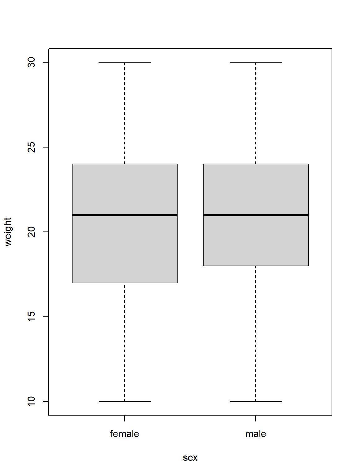
What about potential habitat differences? It makes sense that different habitats, like forests or grasslands or croplands, might have different levels of nutrient availability, or predation pressure, or something that might affect body mass.
# make a boxplot, but turn it horizontal
# and enlarge the y axis margin to make the
# habitat names visible
par(mar=c(4, 10, 1, 1), las=1)
boxplot(weight~habitat, data=dx,
        horizontal = TRUE,
        ylab="", xlab="Body mass (g)")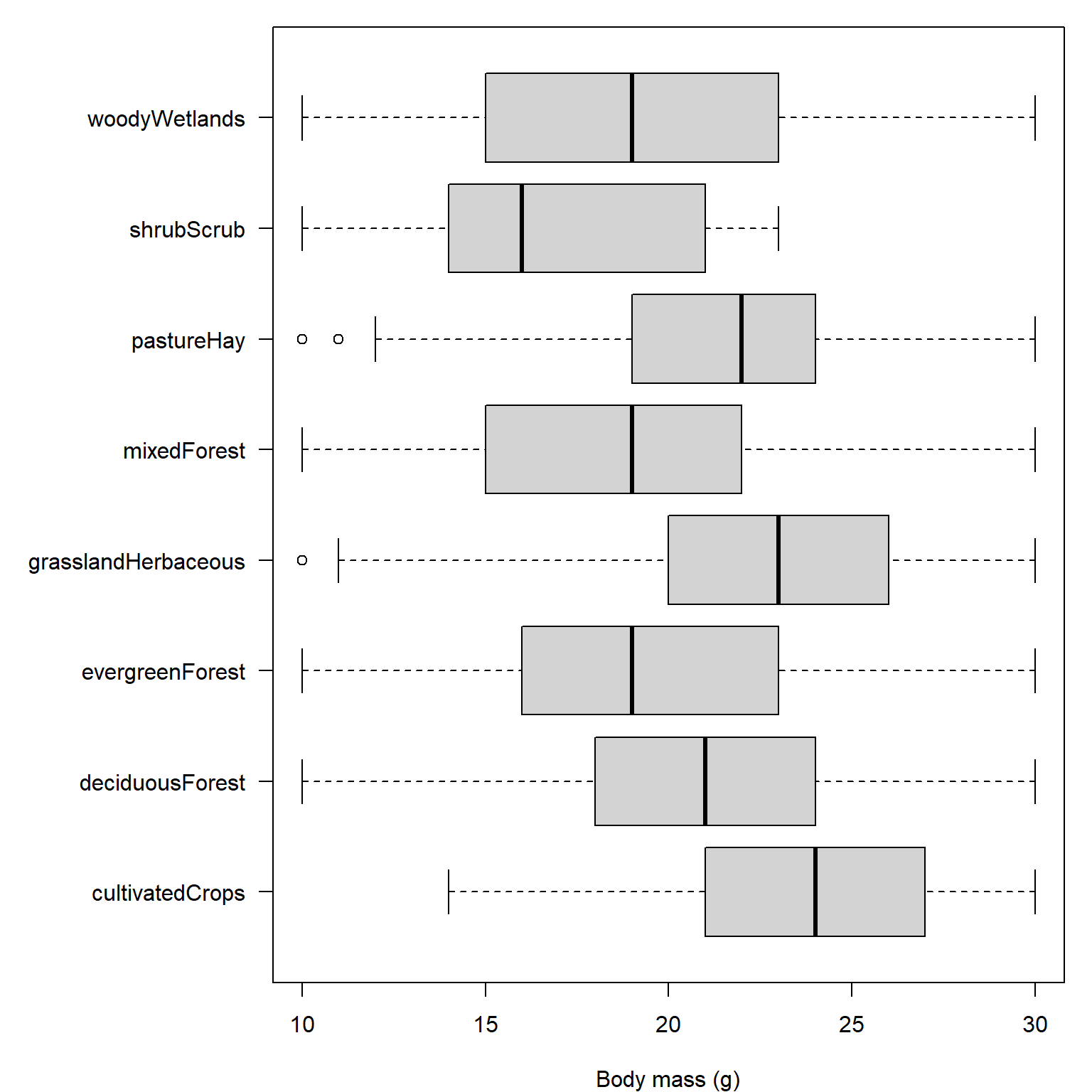
There is a lot of variability, but it looks like there might be some differences in body mass between the habitats.
We will fit the model two ways: as a linear model (two-way ANOVA) and as a linear mixed effects model.
One issue we might want to consider is that each habitat type is represented by several sites, and there might be variability between sites. For example, the “deciduousForest” habitat at GRSM might be different than the same category at HARV. GRSM is in the Great Smoky Mountains National Park in southeastern Tennessee, and HARV is Harvard Forest in Massachusetts. Both are dominated by deciduous forest, but they are not the same kind of deciduous forest. GRSM is in the Ridge and Valley and Southwestern Appalachian ecoregion, while HARV is in the Northeastern Coastal Zone.
We want to isolate the effect of habitat while accounting for other differences between the sites. We need to account for site-to-site variability, but recognize that we are not interested in these sites in and of themselves. The sites where “deciduous forest” and “grassland” were sampled are essentially a random sample of all the many possible places where they could have been sampled. That argues for treating site as a random effect.
The table below shows that deciduous forest and grasslands are each represented by more than 1 site. If we included a habitat represented by only one site, then any apparent effect of that habitat would actually be confounded with that site.
table(dx$habitat, dx$site, useNA="ifany")
                      BART BLAN CLBJ DCFS DELA GRSM HARV JERC JORN KONA KONZ
  cultivatedCrops        0    0    0    0    0    0    0    0    0  121    0
  deciduousForest        0    0    0    0    0 1141 2233    0    0    0    0
  evergreenForest        0    0    0    0    0    0    0    4    0    0    0
  grasslandHerbaceous    0    0  695   14    0    0    0    0    0    0 1744
  mixedForest          465    0    0    0    0    0    0    0    0    0    0
  pastureHay             0 1928    0    0    0    0    0    0    0    0    0
  shrubScrub             0    0    0    0    0    0    0    0    4    0    0
  woodyWetlands          0    0    0    0   81    0    0    0    0    0    0

                      LENO MLBS NOGP OAES ORNL SCBI SERC SRER STEI TALL TREE
  cultivatedCrops        0    0    0    0    0    0    0    0    0    0    0
  deciduousForest        0 1449    0    0 2929 3885 1602    0 1303    0    0
  evergreenForest        0    0    0    0    0    0    0    0    0  464    0
  grasslandHerbaceous    0    0  238  139    0    0    0    0    0    0    0
  mixedForest            0    0    0    0    0    0    0    0    0    0  814
  pastureHay             0    0    0    0    0    0    0    0    0    0    0
  shrubScrub             0    0    0    0    0    0    0    3    0    0    0
  woodyWetlands          6    0    0    0    0    0    0    0    0    0    0

                      UKFS UNDE WOOD
  cultivatedCrops        0    0    0
  deciduousForest     1221    0    0
  evergreenForest        0    0    0
  grasslandHerbaceous    0    0    1
  mixedForest            0    0    0
  pastureHay             0    0    0
  shrubScrub             0    0    0
  woodyWetlands          0  691    0
It looks like we will get the most robust comparison if we restrict our analysis to deciduous forest and grassland habitats. Filter the dataset to those habitats.
# restrict to deciduous forest and grasslands
dx2 <- dx[dx$habitat %in% c("deciduousForest", "grasslandHerbaceous"),]

# remove site wood, which has only 1 animal
dx2 <- dx2[dx2$site != "WOOD",]
Now let’s run the analysis in two ways: as a linear model and as a linear mixed effects model. The linear model version of the analysis is a two-way ANOVA with habitat and sex plus the interaction between them. The mixed model version has the same fixed effects structure, plus a random intercept for site.
library(lme4)
library(lmerTest)

# two-way anova (linear model)
mod1 <- aov(weight~habitat*sex, data=dx2)

# mixed model with random intercept by site
mod2 <- lmer(weight~habitat*sex+(1|site), data=dx2)
Now compare the model fits. The linear version found significant effects of both habitat and sex. The post-hoc test shows that grassland mice were about 2.04 g larger than forest mice and that males were about 0.6 g larger on average females. That’s a big difference (if you’re a mouse).
summary(mod1) Df Sum Sq Mean Sq F value Pr(>F)
habitat 1 9980 9980 569.35 < 2e-16 ***
sex 1 1944 1944 110.93 < 2e-16 ***
habitat:sex 1 208 208 11.84 0.000581 ***
Residuals 18589 325843 18
---
Signif. codes: 0 '***' 0.001 '**' 0.01 '*' 0.05 '.' 0.1 ' ' 1anova(mod2, type=2)Type II Analysis of Variance Table with Satterthwaite's method
Sum Sq Mean Sq NumDF DenDF F value Pr(>F)
habitat 6.06 6.06 1 11.6 0.369 0.5553
sex 1792.84 1792.84 1 18581.5 109.166 < 2.2e-16 ***
habitat:sex 289.13 289.13 1 18588.2 17.605 2.732e-05 ***
---
Signif. codes: 0 '***' 0.001 '**' 0.01 '*' 0.05 '.' 0.1 ' ' 1Interestingly, the main effect of habitat is significant in the linear model, but not in the mixed model.
anova(mod2, type=2)Type II Analysis of Variance Table with Satterthwaite's method
Sum Sq Mean Sq NumDF DenDF F value Pr(>F)
habitat 6.06 6.06 1 11.6 0.369 0.5553
sex 1792.84 1792.84 1 18581.5 109.166 < 2.2e-16 ***
habitat:sex 289.13 289.13 1 18588.2 17.605 2.732e-05 ***
---
Signif. codes: 0 '***' 0.001 '**' 0.01 '*' 0.05 '.' 0.1 ' ' 1In the random intercept model (mod2), the effect of habitat–which significant in the ANOVA–was nonsignificant and only the effect of sex remains. What happened? It appears that some of the variance that was previously attributed to habitat appears to now be associated with site.
There appears to be an interaction between sex and habitat. Let’s check the coefficients:
coef(mod1) (Intercept) habitatgrasslandHerbaceous
20.5895575 1.6560410
sexmale habitatgrasslandHerbaceous:sexmale
0.5629499 0.5987715 The output tells us that females in grasslands are, on average, 1.65 g larger than females in deciduous forests, while males in deciduous forests are, on average, 0.56 g larger than females in deciduous forests. However, the difference between males and females is greater in grasslands (0.56 + 0.60 = 1.16 g). The interaction coefficient (0.60 g) represents the additional difference between male and female body mass in grasslands compared with deciduous forests. What about in the random intercept model?
fixef(mod2) (Intercept) habitatgrasslandHerbaceous
20.77687386 0.04660303
sexmale habitatgrasslandHerbaceous:sexmale
0.52194319 0.71051491 In this model, females in grassland are not significantly larger than females in deciduous forest (0.046). This is different than the linear model. The other findings are similar to the linear model:mMales in deciduous forest are about 0.52 g larger than females in deciduous forest, while in grasslands, the difference between males and females is about 0.123 (0.52+0.71).
We can see the random effects with ranef(). These value are the deviations of each group-level intercept and slope from the global intercept of 20.77.
# these are deviations from population-level parameters
re3 <- ranef(mod2)
re3$site
(Intercept)
CLBJ -0.05596660
DCFS -0.72368354
GRSM -0.54512707
HARV -0.06942544
KONZ 2.43867916
MLBS -0.31408447
NOGP -0.69340088
OAES -0.96562814
ORNL -1.41879991
SCBI -0.05249160
SERC 0.29511656
STEI -0.55544391
UKFS 2.66025583The random effects should have mean 0 and an SD corresponding to the variances reported by summary(mod2) (up to sampling error). We can get the actual variances with VarCorr().
# estimated variances, standard deviations,
# and correlations of random effects
VarCorr(mod2)
Groups Name Std.Dev.
site (Intercept) 1.3008
Residual 4.0525 Finally, we can see the group-specific coefficients, which include the fixed and the random effect, with coef(). Notice that only the intercepts vary between sites. If we had specified random effects of habitat or sex, those columns would vary as well.
# group-specific coefficients (fixed + random effects)
# these are the group-specific coefficients themselves
coef(mod2)
$site
(Intercept) habitatgrasslandHerbaceous sexmale
CLBJ 20.72091 0.04660303 0.5219432
DCFS 20.05319 0.04660303 0.5219432
GRSM 20.23175 0.04660303 0.5219432
HARV 20.70745 0.04660303 0.5219432
KONZ 23.21555 0.04660303 0.5219432
MLBS 20.46279 0.04660303 0.5219432
NOGP 20.08347 0.04660303 0.5219432
OAES 19.81125 0.04660303 0.5219432
ORNL 19.35807 0.04660303 0.5219432
SCBI 20.72438 0.04660303 0.5219432
SERC 21.07199 0.04660303 0.5219432
STEI 20.22143 0.04660303 0.5219432
UKFS 23.43713 0.04660303 0.5219432
habitatgrasslandHerbaceous:sexmale
CLBJ 0.7105149
DCFS 0.7105149
GRSM 0.7105149
HARV 0.7105149
KONZ 0.7105149
MLBS 0.7105149
NOGP 0.7105149
OAES 0.7105149
ORNL 0.7105149
SCBI 0.7105149
SERC 0.7105149
STEI 0.7105149
UKFS 0.7105149
attr(,"class")
[1] "coef.mer"If desired, you can also get confidence intervals of the fixed effects with confint(). This can take a while depending on the number of observations and the complexity of the model.
# confidence intervals
# this can take a minute
confint(mod2)
2.5 % 97.5 %
.sig01 0.8372966 1.8776447
.sigma 4.0114561 4.0938633
(Intercept) 19.8751759 21.6788283
habitatgrasslandHerbaceous -1.4714719 1.5441645
sexmale 0.3944790 0.6494902
habitatgrasslandHerbaceous:sexmale 0.3784273 1.0421999We can see that the fixed effect of habitat is indeed different than the corresponding main effect in the linear model:
confint(mod1) 2.5 % 97.5 %
(Intercept) 20.4916749 20.6874402
habitatgrasslandHerbaceous 1.3936223 1.9184598
sexmale 0.4314520 0.6944478
habitatgrasslandHerbaceous:sexmale 0.2577007 0.9398422We can calculate 95% CI for the random coefficients, but we need to be careful here. Remember that a random effect allows us to account for variability between sites, but does not allow us to make inferences about the differences between sites. If we want to do that, we need to fit site as a fixed effect. Still, inspecting the coefficients can often give us a clue about the structure of variation in our dataset.
# to get the 95% CI estimate of the random coefficients:
## extract conditional variances (to go along with conditional modes)
re <- ranef(mod2, condVar = TRUE)

##  pull values as numeric
b <- re$site[, 1]

## convert to SE (sqrt of var)
se <- sqrt(attr(re$site, "postVar")[1, 1, ])

## assemble in data frame and estimate CI
## note that these are the effects from
## the population-level value. Add fixef(mod2)[1]
## to get estimate and 95% CI of conditional modes
cond.ci <- data.frame(
    site = rownames(re$site),
    estimate = b,
    lower = b - 1.96 * se,
    upper = b + 1.96 * se
)
cond.ci
site estimate lower upper
1 CLBJ -0.05596660 -0.3551784 0.24324526
2 DCFS -0.72368354 -2.3550468 0.90767975
3 GRSM -0.54512707 -0.7792806 -0.31097359
4 HARV -0.06942544 -0.2371500 0.09829912
5 KONZ 2.43867916 2.2490066 2.62835169
6 MLBS -0.31408447 -0.5220536 -0.10611531
7 NOGP -0.69340088 -1.1980788 -0.18872294
8 OAES -0.96562814 -1.6169837 -0.31427255
9 ORNL -1.41879991 -1.5653226 -1.27227726
10 SCBI -0.05249160 -0.1797673 0.07478411
11 SERC 0.29511656 0.0972648 0.49296833
12 STEI -0.55544391 -0.7746735 -0.33621436
13 UKFS 2.66025583 2.4338406 2.88667108It might be more helpful to plot the random effects:
lattice::dotplot(ranef(mod2, condVar = TRUE))$site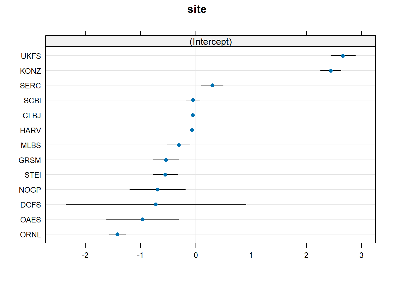
23.2.3 Specifying random effects in lme4
In lme4, the random effects are added to a model formula as terms after the fixed effects. Random effects are added in a form like (a|b), where a defines the model term that is a random effect, and b is the factor that defines the groups. The syntax for random effects models differs slightly between the two most popular mixed models packages, lme4 and nlme. The table below shows some example random effects structures in lme4:
lme4.
| Formula | Meaning |
|---|---|
(1 | g) |
Random intercept for each level of grouping variable g. |
(1 | g1/g2) |
Random intercepts for g1 and for g2 nested within g1. Equivalent to (1 | g1) + (1 | g1:g2). |
(1 | g1) + (1 | g2) |
Random intercepts for two grouping variables, typically crossed rather than nested. |
(x | g) |
Random intercept and random slope for x by g. Their correlation is estimated. |
(x || g) |
Random intercept and random slope for numeric x by g, with their correlation constrained to zero. May help with convergence or singular fits. |
(0 + x | g) |
Random slope for x by g, without a random intercept for g. |
You can define a huge variety of random effects structures, but probably shouldn’t. As with defining potential regression models or GLMs, it is incumbent on you as a biologist to think critically about what models represent biologically reasonable hypotheses.
23.3 Generalized linear mixed effects models (GLMM)
Just as generalized linear model (GLM) extend linear models by allowing for non-normal response distributions, generalized linear mixed models (GLMM) extend linear mixed models in the same way. We will use package lme4 to fit GLMM.
23.3.1 Definition
The overall structure of a GLMM is similar to the structure of a GLM. The only difference is that while the only variance component of a GLM is in the response distribution (and thus relates to residual variation), GLMMs add additional structure to the variance by allowing model parameters to vary randomly.
The response variable \(y\) varies according to some distribution with expected value \(E\left(y\right)\) and sometimes additional parameters \(\theta\):
\[y\sim SomeDistribution\left(E\left(y\right),\theta\right)\]
The expected value on the data scale is related to the scale of the linear predictor \(\eta\) by a link function:
\[\text{LinkFunction}\left(E\left(y\right)\right)=\eta\]
And the linear predictor \(\eta\) is a linear function of the predictor variables (we’ll just use 1, \(x\), for now).
\[\eta=\beta_0+\beta_1 x\]
But, to make this a GLMM instead of a GLM, we let the model parameters vary according to levels of some factor (grouping variable) denoted by \(j\). For example, a GLM with a random intercept will have linear predictor
\[\eta=\beta_{0,j}+\beta_1 x\]
\[\beta_0\sim\mathcal{Normal}\left(\mu_{\beta_0},\sigma^2_{\beta_0}\right)\]
and a GLM with a random slope will look like
\[\eta=\beta_0+\beta_{1,j} x\]
\[\beta_1\sim\mathcal{Normal}\left(\mu_{\beta_1},\sigma^2_{\beta_1}\right)\]
And remember, as with LME, we can write the means (or coefficients) parameterization as above where \(\beta_0\) or \(\beta_1\) follow distributions, or we can write the effects (or deviation) parameterization where the global parameter is specified and we fit the variance of the random effects. For example:
\[\eta=\left(\beta_0+\gamma_j\right)+\beta_1 x\]
\[\gamma_j\sim\mathcal{Normal}\left(0,\sigma^2_{\beta_0}\right)\]
In the means parameterization, we fit \(\mu_{\beta_k}\) as the global intercept (or slope) and the variance \(\sigma^2_{\beta_k}\) to define the spread among the groups. In the effects parameterization, we fit the global intercept or slope (i.e., the fixed effect) as \(\beta_k\), and assume that group-level values vary according to a normal distribution with mean 0 and variance \(\sigma^2_{\beta_k}\). The effects parameterization is what R and lme4 present by default, but I find it more informative to write and discuss the model in means parameterization. Your mileage may vary.
To summarize: in the effects parameterization, we model how much each group differs from the population-level intercept; in the means parameterization, we model the group-specific intercepts directly. Both describe the same model, and we can translate between them by adding or subtracting the population-level intercept.
The difference between these two modes of specifying group-level parameters is shown in Table 23.2 below.
| Quantity | Effects parameterization | Means parameterization |
|---|---|---|
| Population-level intercept | \(\beta_0\) | \(\mu_{\beta_0}\) |
| Group-level quantity | \(\gamma_j\) | \(\beta_{0j}\) |
| Distribution | \(\gamma_j \sim N(0,\sigma_{\beta_0}^2)\) | \(\beta_{0j} \sim N(\mu_{\beta_0},\sigma_{\beta_0}^2)\) |
| Group-specific intercept | \(\beta_0+\gamma_j\) | \(\beta_{0j}\) |
lme4 extraction |
ranef(mod) |
coef(mod) |
23.3.2 Example with NEON data
23.3.2.1 Data import and first steps
Let’s revisit the NEON small mammal capture data. Download the individual measurement dataset and the taxonomic dataset and put them in your working directory.
tax <- read.csv("data-neon-taxa.csv")
ind <- read.csv("data-neon-ind-meas.csv")
We are going to use mixed models to investigate sexual dimorphism in body mass in white-footed mice (Peromyscus leucopus). We investigated this previously in Section 23.2.2. This time, we are going to investigate how body mass varies with body length in males and females. We are going to use a Gaussian GLM with a log-link. The log-link is appropriate here because body mass is a strictly positive, continuous variable. However, we do not suspect overdispersion, so we don’t need a Gamma distribution. We will also test a random effect for site. We are interested in this random effect because different sites have different conditions that may affect body mass.
First, filter the data down to P. leucopus, with non-missing weights and lengths, with realistic masses and lengths, and with known sex.
# filter to species P. leucopus
dx <- ind[ind$abb == "Perleu",]

# only need these columns
dx <- dx[,c("tagID", "sex", "totalLength", "weight")]

# drop missing measurements
dx <- dx[complete.cases(dx),]

# realistic weights, probably correct
dx <- dx[dx$weight > 10 & dx$weight < 30,]

# realistic adult lengths
dx <- dx[dx$totalLength > 80,]

# drop unknown sex
sexes <- c("female", "male")
dx <- dx[dx$sex %in% sexes,]

# extract site
dx$site <- sapply(strsplit(dx$tagID, "_"), "[", 2)

# symbology
cols <- c("red", "blue")
pchs <- c(16,17)
names(cols) <- names(pchs) <- sexes
dx$pch <- pchs[dx$sex]
dx$col <- cols[dx$sex]
At first glance, it appears that mass increases with total length (as it should). It’s hard to tell whether there is an effect of sex. We should suspect from Section 23.2.2 that there is at least a main effect of sex (different intercept).
par(mar=c(5,5,1,1))
plot(weight~totalLength, data=dx,
        pch=dx$pch, col=dx$col,
        ylab="Body mass (g)", log="xy",
        ylim=c(10, 30))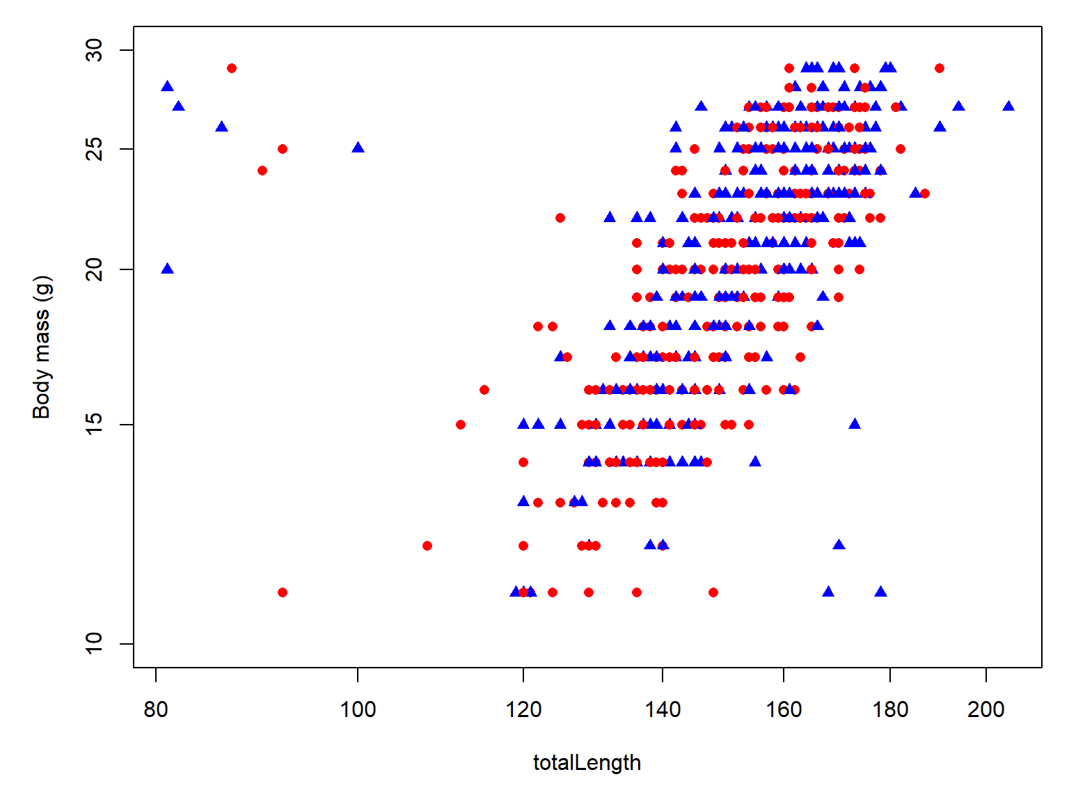
It looks like there are some anomalous points in the upper left of the plots. Mice up there have very large mass relative to their body length. Let’s delete them and replot.
dx <- dx[dx$totalLength > 102,]

par(mar=c(5,5,1,1))
plot(weight~totalLength, data=dx,
        pch=dx$pch, col=dx$col,
        ylab="Body mass (g)", log="xy",
        ylim=c(10, 30))
legend("right", legend=sexes,pch=pchs,col=cols)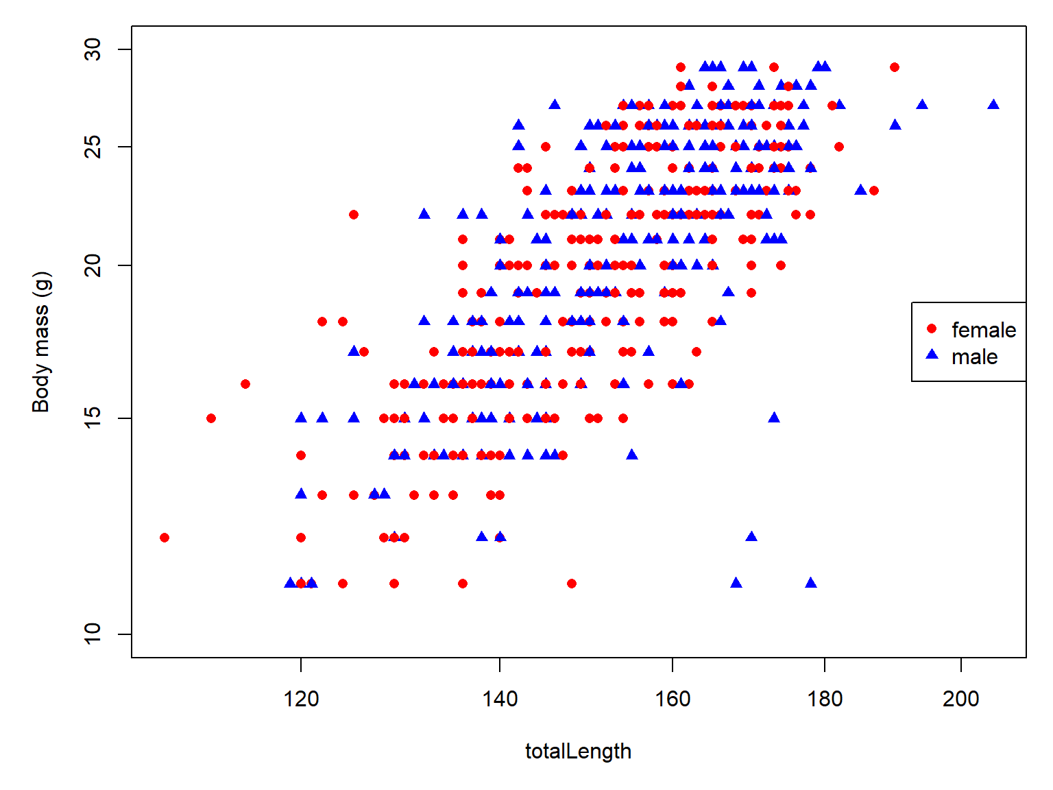
Much better. Those anomalous mice might be legitimate–for example, a mouse with an injured or missing tail would have a very large mass relative to its total length–but that would still warrant their removal.
23.3.2.2 Fit GLM and GLMMM
Now Let’s fit a GLM and a GLMM version of our model.
dx$loglen <- log(dx$totalLength)

mod04 <- glm(weight~loglen+sex,
               data=dx, family=gaussian(link="log"))
summary(mod04)
Call:
glm(formula = weight ~ loglen + sex, family = gaussian(link = "log"),
    data = dx)

Coefficients:
            Estimate Std. Error t value Pr(>|t|)
(Intercept) -5.30436    0.33202 -15.976   <2e-16 ***
loglen       1.65159    0.06578  25.107   <2e-16 ***
sexmale      0.02187    0.01254   1.743   0.0818 .
---
Signif. codes:  0 '***' 0.001 '**' 0.01 '*' 0.05 '.' 0.1 ' ' 1

(Dispersion parameter for gaussian family taken to be 9.52346)

    Null deviance: 12166.2  on 572  degrees of freedom
Residual deviance:  5428.4  on 570  degrees of freedom
AIC: 2922.5

Number of Fisher Scoring iterations: 4
The results suggest that body length actually accounts for more variation in body mass than sex does. Let’s add the random effect for site and refit as a GLMM. We are going to use an alternative optimizer because the default optimizer had an issue with convergence diagnostics. Different optimizers sometimes produce convergence warnings even when they arrive at essentially the same maximum-likelihood estimates. Comparing optimizers is one way to diagnose these warnings
library(lme4)

mod05 <- glmer(weight~loglen+sex+(1|site),
               data=dx, family=gaussian(link="log"),
               control = glmerControl(optimizer = "bobyqa",
                                      optCtrl = list(maxfun = 2e5))
               )
summary(mod05)
Generalized linear mixed model fit by maximum likelihood (Laplace
Approximation) [glmerMod]
Family: gaussian ( log )
Formula: weight ~ loglen + sex + (1 | site)
Data: dx
Control: glmerControl(optimizer = "bobyqa", optCtrl = list(maxfun = 2e+05))
AIC BIC logLik -2*log(L) df.resid
2894.7 2916.4 -1442.3 2884.7 568
Scaled residuals:
Min 1Q Median 3Q Max
-4.5609 -0.6994 -0.0369 0.6202 2.7373
Random effects:
Groups Name Variance Std.Dev.
site (Intercept) 0.007231 0.08504
Number of obs: 573, groups: site, 12
Fixed effects:
Estimate Std. Error t value Pr(>|z|)
(Intercept) -5.25130 0.34948 -15.03 <2e-16 ***
loglen 1.64650 0.06901 23.86 <2e-16 ***
sexmale 0.02639 0.01210 2.18 0.0293 *
---
Signif. codes: 0 '***' 0.001 '**' 0.01 '*' 0.05 '.' 0.1 ' ' 1
Correlation of Fixed Effects:
(Intr) loglen
loglen -0.996
sexmale 0.077 -0.097The fixed effects are pretty similar, and the AICs suggest that adding the random effect improved the model. Interestingly, the fixed effect of sex is statistically significant in the GLMM version of the model. Variance that was attributed to residual variation in the GLM was soaked up by random effect of site, which helped us detect the sex effect that we had every reason to expect to see.
Let’s compare the models by AIC:
AIC(mod04, mod05) df AIC
mod04 4 2922.499
mod05 5 2894.660The GLMM version has a much lower AIC, suggesting that including the random effect yields a model with better support.
23.3.2.3 Plotting population-level predictions
Let’s plot the model’s predicted values to see how male and female mouse mass varies with length.
# sex-specific sequences of x values
px1 <- seq(min(dx$loglen[dx$sex=="female"]),
           max(dx$loglen[dx$sex=="female"]), length=100)
px2 <- seq(min(dx$loglen[dx$sex=="male"]),
           max(dx$loglen[dx$sex=="male"]), length=100)

# sex-specific data frames
prx1 <- data.frame(loglen=px1, length=exp(px1), sex="female")
prx2 <- data.frame(loglen=px2, length=exp(px2), sex="male")
When we calculate predictions, we need to use the argument re.form to specify how predict() will account for the random effects. We will use re.form=NA, which gives us the population-level prediction with the random effects set to 0. In other words, this is the predicted value at the average random effect on the link scale. It does not represent a prediction averaged over the distribution of random effects across sites (i.e., the marginal mean). To obtain that, we must account for the estimated variance of the random effects. With an identity link function, these two predictions are the same. With a nonlinear link function such as the logarithmic link used here, the difference can be substantial, especially if the random-effect variance is large.
The take-home message is that re.form=NA is appropriate for illustrating the fixed-effect relationship, but we should be careful not to refer to these predictions as population-averaged means. In summary:
- Population-level prediction with the random effects set to 0: Expected mass at a site with random intercept zero. Set
re.form=NA. - Marginal means (population average): Expected mass averaged over the distribution of site random effects. Need to integrate over random effects (see example below).
# calculate population-level predictions
prx1$fit <- predict(mod05, newdata = prx1,
                    type = "response", re.form = NA)

prx2$fit <- predict(mod05, newdata = prx2,
                    type = "response", re.form = NA)
And plot:
par(mar=c(5,5,1,1))
plot(weight~totalLength, data=dx,
        pch=dx$pch, col=dx$col,
        ylab="Body mass (g)", log="xy",
        ylim=c(10, 50))
lines(prx1$length, prx1$fit, col=cols[1], lwd=3)
lines(prx2$length, prx2$fit, col=cols[2], lwd=3)
legend("right", legend=sexes,
       pch=pchs, col=cols, lwd=3)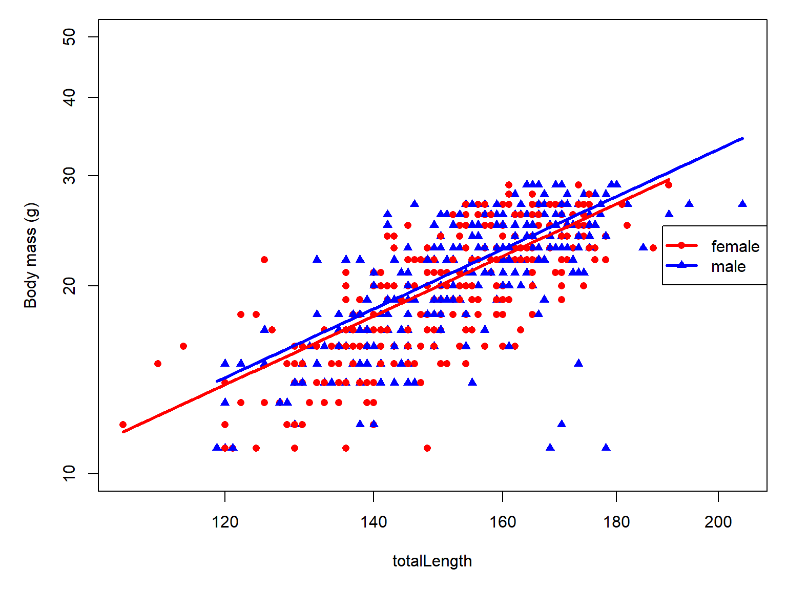
Finally, let’s calculate and present the 95% confidence intervals. Unlike glm() and lm(), glmer() does not provide se.fit=TRUE in the usual way. There are two reasonable approaches.
For the population-level predictions, we can calculate the standard error of the linear predictor using the fixed-effect variance-covariance matrix, then transform the confidence limits back to grams.
get_ci <- function(mod, newdata) {

  newdata$sex <- factor(newdata$sex,
                        levels = levels(model.frame(mod)$sex))

  X <- model.matrix(
    delete.response(terms(mod, fixed.only = TRUE)),
    data = newdata
  )

  b <- fixef(mod)
  V <- as.matrix(vcov(mod))

  eta <- as.vector(X %*% b)
  se <- sqrt(rowSums((X %*% V) * X))

  newdata$fit.plm <- exp(eta)
  newdata$lwr.plm <- exp(eta - 1.96 * se)
  newdata$upr.plm <- exp(eta + 1.96 * se)

  newdata
}

prx3 <- rbind(prx1, prx2)
prx3 <- get_ci(mod05, prx3)
head(prx3)
loglen length sex fit fit.plm lwr.plm upr.plm
1 4.682131 108.0000 female 11.67928 11.67928 10.80264 12.62706
2 4.687837 108.6180 female 11.78952 11.78952 10.90987 12.74010
3 4.693543 109.2396 female 11.90080 11.90080 11.01811 12.85422
4 4.699249 109.8647 female 12.01314 12.01314 11.12737 12.96941
5 4.704955 110.4933 female 12.12653 12.12653 11.23766 13.08571
6 4.710661 111.1256 female 12.24100 12.24100 11.34899 13.20311And check out the plot:
par(mar=c(5,5,1,1))
plot(weight~totalLength, data=dx,
        pch=dx$pch, col=dx$col,
        ylab="Body mass (g)", log="xy",
        ylim=c(10, 50))
flag <- which(prx3$sex=="female")
lines(prx3$length[flag], prx3$fit.plm[flag],
      col=cols[1], lwd=3)
lines(prx3$length[flag], prx3$lwr.plm[flag],
      col=cols[1], lwd=3, lty=2)
lines(prx3$length[flag], prx3$upr.plm[flag],
      col=cols[1], lwd=3, lty=2)

flag <- which(prx3$sex=="male")
lines(prx3$length[flag], prx3$fit.plm[flag],
      col=cols[2], lwd=3)
lines(prx3$length[flag], prx3$lwr.plm[flag],
      col=cols[2], lwd=3, lty=2)
lines(prx3$length[flag], prx3$upr.plm[flag],
      col=cols[2], lwd=3, lty=2)
legend("top", legend=sexes,
       pch=pchs, col=cols, lwd=3)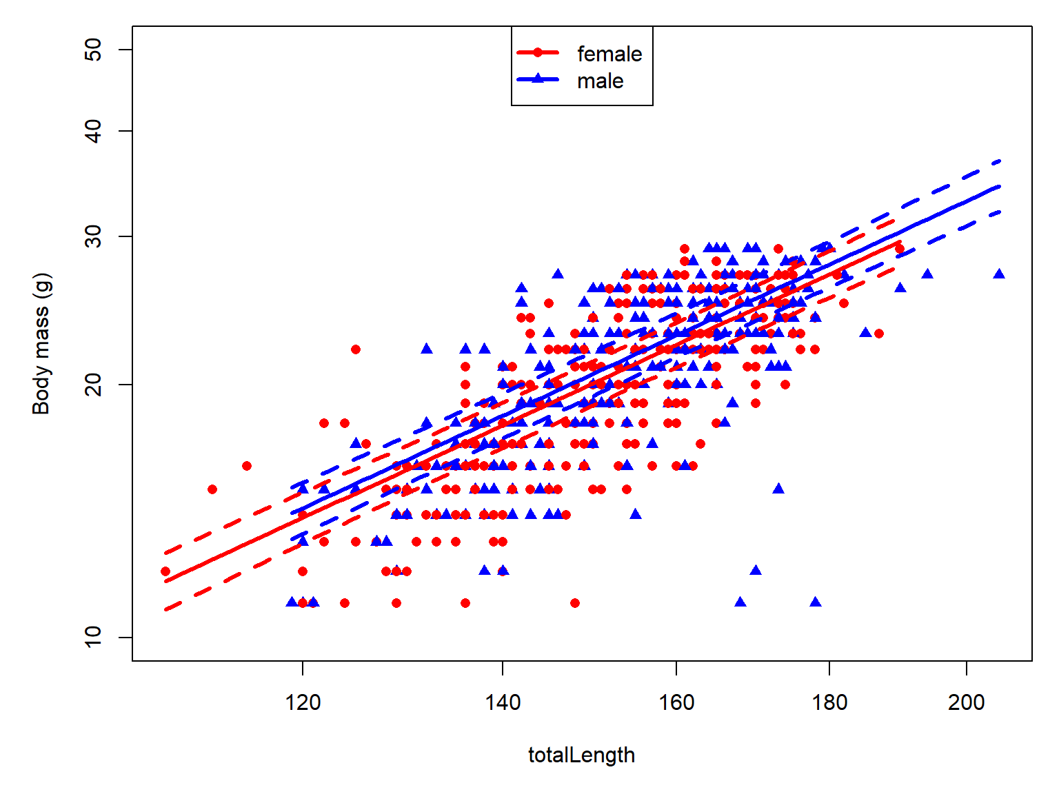
23.3.2.4 Plotting marginal means
If we want to see the marginal means, which are predictions that average over the distribution of sites, we need to integrate over the distribution of random effects. Note that the calculations below are specific to this model, a Gaussian GLM(M) with a log link. If you have a different response distribution or link function, the calculation is different.
v <- as.numeric(VarCorr(mod05)$site[1, 1])

prx1$fit.mm <- predict(mod05,
                       newdata = prx1,
                       type = "response", re.form = NA) *
    exp(v / 2)

prx2$fit.mm <- predict(mod05,
                       newdata = prx2,
                       type = "response", re.form = NA) *
    exp(v / 2)


par(mar=c(5,5,1,1))
plot(weight~totalLength, data=dx,
        pch=dx$pch, col=dx$col,
        ylab="Body mass (g)", log="xy",
        ylim=c(10, 50))
lines(prx1$length, prx1$fit.mm, col=cols[1], lwd=3)
lines(prx2$length, prx2$fit.mm, col=cols[2], lwd=3)
legend("topleft", legend=sexes,
       pch=pchs, col=cols, lwd=3, bty="n")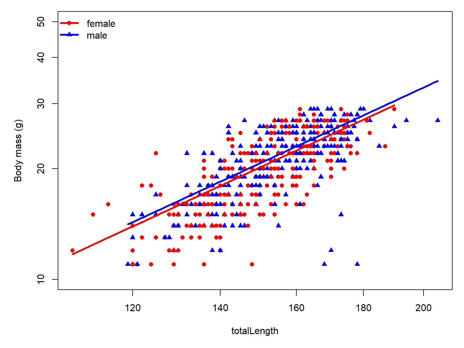
In this case, the marginal means and the population-level predictions are pretty similar. Note that the procedure above is appropriate for a Gaussian GLMM with a log-link. The integration is different for other GLMMs.
We can also plot the 95% CI of the marginal means, but it’s a little more involved. One way to estimate the CI is to use a parametric bootstrap using bootMER(). The code block below was not run during rendering because it takes over an hour.
pred_fun <- function(mod) {
  v <- as.numeric(VarCorr(mod)$site[1, 1])
  predict(mod, newdata = prx3,
          type = "response", re.form = NA) * exp(v / 2)
}

set.seed(123)

bt <- bootMer(mod05, FUN = pred_fun,
              nsim = 500, type = "parametric",
              use.u = FALSE)

prx3$fit.boot <- pred_fun(mod05)
prx3$lwr.boot <- apply(bt$t, 2, quantile,
                       0.025, na.rm = TRUE)
prx3$upr.boot <- apply(bt$t, 2, quantile,
                       0.975, na.rm = TRUE)

# then make the plot as usual
23.4 Nonlinear mixed effects models
Coming soon!
23.4.1 Definition
23.4.2 Example with NEON data
23.4.3 Specifying random effects in nlme
23.5 Additive mixed models (GAMM)
Coming soon!