In a test for difference in mean or location, we are interested in whether observations differ between groups. Most of the time we are testing whether the central tendency differs between groups. A test of this kind evaluates a prediction like, “a typical value in group A is different from a typical value in group B”.
Alternatively, we can test for a difference in location: the relative position of random values from 2 or more groups. This is a slightly different statement: “values in group A tend to be greater than (or less than) values in group B”. Put another way: “If we pick a random value from group A, it will be reliably greater (or less than) than a random value from group B”. Tests for location are performed on the rank order of the values, not the values themselves.
When comparing groups, the data are usually best shown using a boxplot, also known as a box-and-whiskers plot. The exact implementation varies between software packages, but boxplots usually show the median, interquartile range (approximately), extreme values, and possible outliers (if any) Run the command ?boxplot.stats to see a description of how boxplots are calculated in R.
15.1 Tests for 1 group
When all of the values come from the same set of observations, we can ask questions such as:
Is the mean in this group equal to, or different from, some arbitrary value?
Is the mean in this group greater than, or not greater than, some arbitrary value?
These questions are the domain of one-sample tests. The most important is the one-sample t-test, which comes in two varieties: one-tailed and two-tailed. All one-sample tests compare the mean of a set of values to some quantity (hypothetical mean) of interest, called \(\mu\) (the Greek letter “mu”). In a one-tailed test, the null hypothesis is that the underlying population mean is either \(\le\mu\) or \(\ge\mu\). In a two-tailed test, the null hypothesis is that the population mean is equal to \(\mu\).
A note on symbology: sample vs. population parameters
In statistics, we analyze samples (randomly-selected subsets of observed entities) to make inferences about populations (the hypothetical set of all possible entities which could be included in a sample). For example, if you wanted to know how the population of a nation of 100 million citizens felt about some political issue, it would be time-consuming and expensive to ask each citizen what they thought. Instead, you would sample a randomly selected set of 1000 citizens and then assume that those results reflected the opinion of the entire citizenry. For this assumption to work, your sample must be both random and representative of the entire population.
Similarly, in science we cannot collect a infinite amount of data, or measure every squirrel in the forest, or any other type of exhaustive and comprehensive data collection. We instead take representative samples of all the possible samples–i.e., the population–and rely on good practices in experimental design to enable us to assume that our sample represents the population.
The reason I bring this up here is that we need to keep in mind the difference between sample statistics and population statistics. Sample statistics are calculated from your data. Population statistics are inferred from your data using statistical models. This is why statistical tests are commonly referred to as inferential statistics, and why simple calculations from data are referred to as descriptive statistics.
The most common descriptive statistics are shown below:
Parameter
Sample
Population
Mean
\(\bar{x}\)
\(\mu\)
Variance
\(s^{2}\)
\(\sigma^{2}\)
Standard deviation
\(s\)
\(\sigma\)
15.1.1 One-sample, one-tailed t-test
In a one-tailed one-sample test, we are interested in whether the underlying population mean (\(\mu\)) of a set of values is not equal to some value of interest…either at most some value, or at least some value.
Question: Is the mean value less than OR greater than some value \(x\)?
Null hypothesis: True mean is \(=x\).
Alternative hypothesis: True mean is \(<x\) or true mean is \(>x\).
Example use case:Fred needs to check whether the mean measurement error across his 12 technicians is less than 0.5 mm.
Here is an example where we simulate some data in R and run a one-tailed one-sample t-test.
# simulate some values with nominal mean 5 and sd 3set.seed(123)a <-rnorm(20, 5, 3)# 1 sample 1 tailed t-test# Example 1: Is the underlying mean <= 0?t.test(a, alternative="greater")
    One Sample t-test

data:  a
t = 8.3142, df = 19, p-value = 4.707e-08
alternative hypothesis: true mean is greater than 0
95 percent confidence interval:
 4.29664     Inf
sample estimates:
mean of x
 5.424871
# Example 2: Is the underlying mean <= 4?t.test(a, alternative="greater", mu=4)
    One Sample t-test

data:  a
t = 2.1838, df = 19, p-value = 0.02086
alternative hypothesis: true mean is greater than 4
95 percent confidence interval:
 4.29664     Inf
sample estimates:
mean of x
 5.424871
Interpretation: In the example above, the researcher can reject the null hypothesis that the true mean is \(\leq4\), and conclude that the true mean is \(>4\).
# Example 3: Is the underlying mean >= 5.5?t.test(a, alternative="less", mu=5.5)
    One Sample t-test

data:  a
t = -0.11514, df = 19, p-value = 0.4548
alternative hypothesis: true mean is less than 5.5
95 percent confidence interval:
     -Inf 6.553102
sample estimates:
mean of x
 5.424871
Interpretation: In example 3, the researcher cannot reject the null hypothesis that \(\mu\geq5.5\). This makes sense, because the true mean is about \(5.4\pm2.9\) (verify with mean(a);sd(a)).
15.1.2 One-sample, two-tailed t-test
In a two-tailed test, we are interested in whether the underlying population mean of a set of values is equal to some value of interest.
Question: Is the underlying true mean equal to, or different from, some value \(\mu\)?
Null hypothesis: True mean \(=\mu\).
Alternative hypothesis: True mean \(\neq\mu\)
Example use case: Wilma needs to test whether the mean pH of her prepared stock solution is equal to, or different from, the target pH of 7.7.
Here is an example where we simulate some data and conduct a one-sample, two-tailed t-test.
# simulate dataset.seed(123)a <-rnorm(20, 3, 1)# 1 sample 2-tailed t-test:## Example 1: mu = 0 (default)t.test(a)
    One Sample t-test

data:  a
t = 14.445, df = 19, p-value = 1.067e-11
alternative hypothesis: true mean is not equal to 0
95 percent confidence interval:
 2.686402 3.596845
sample estimates:
mean of x
 3.141624
Interpretation: In the example above, the researcher can reject the null that the true mean = 0, and conclude that the true mean is significantly different from 0.
Here’s another example with a different dataset and test.
# simulate dataset.seed(123)a <-rnorm(20, 3, 1)# 1 sample 2-tailed t-test:## Example 2: mu = 5t.test(a, mu=5)
    One Sample t-test

data:  a
t = -8.5445, df = 19, p-value = 6.218e-08
alternative hypothesis: true mean is not equal to 5
95 percent confidence interval:
 2.686402 3.596845
sample estimates:
mean of x
 3.141624
Interpretation: The researcher can reject the null hypothesis that the mean = 5, and conclude that the true mean is not 5. Note that this includes both \(<5\) and \(>5\) as possibilities, but the direction is obvious from the sample mean.
When most people say “t-test”, what they usually mean is a two-sample, two-tailed t-test that tests for a difference in means between two groups. The original version was introduced as the Student’s t-test by William Sealy Gosset in 19081; modern software uses a modified version called the Welch t-test (or sometimes the “Welch-Satterthwaite t-test”, but this is not quite correct). The newer version is better at accounting for non-normality and unequal variances.
The test statistic, t, is basically the difference in sample means scaled by the variance in each group and the sample size in each group. It is calculated as:
\[
t = \frac{\bar{x}_1-\bar{x}_2}
{\sqrt{\frac{s_1^2}{n_1}+\frac{s_2^2}{n_2}}}
\]
where \(\bar{x_1}\) and \(\bar{x_2}\) are the sample means, \(s_1^2\) and \(s_2^2\) are the sample variances, and \(n_1\) and \(n_2\) are the sample sizes. Think through that equation…what would increasing the difference in means (the numerator) do to t? What about increasing one or both sample sizes? One or both sample variances?
Basically, the numerator of t is the quantity of interest: the difference in means between two groups. The denominator is the standard error (SE) of that estimate.
A t value by itself doesn’t tell you much, though, because what we’re interested in is how likely that t score is relative to the number of degrees of freedom (DF) in the dataset. While the early users would simply use n-1 as the DF, modern t-statistics and t distributions are defined by a newer version of the degrees of freedom calculation:
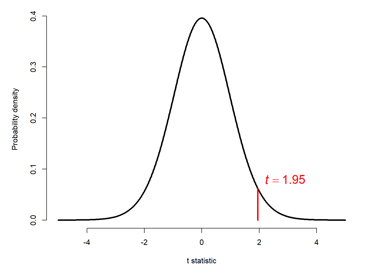
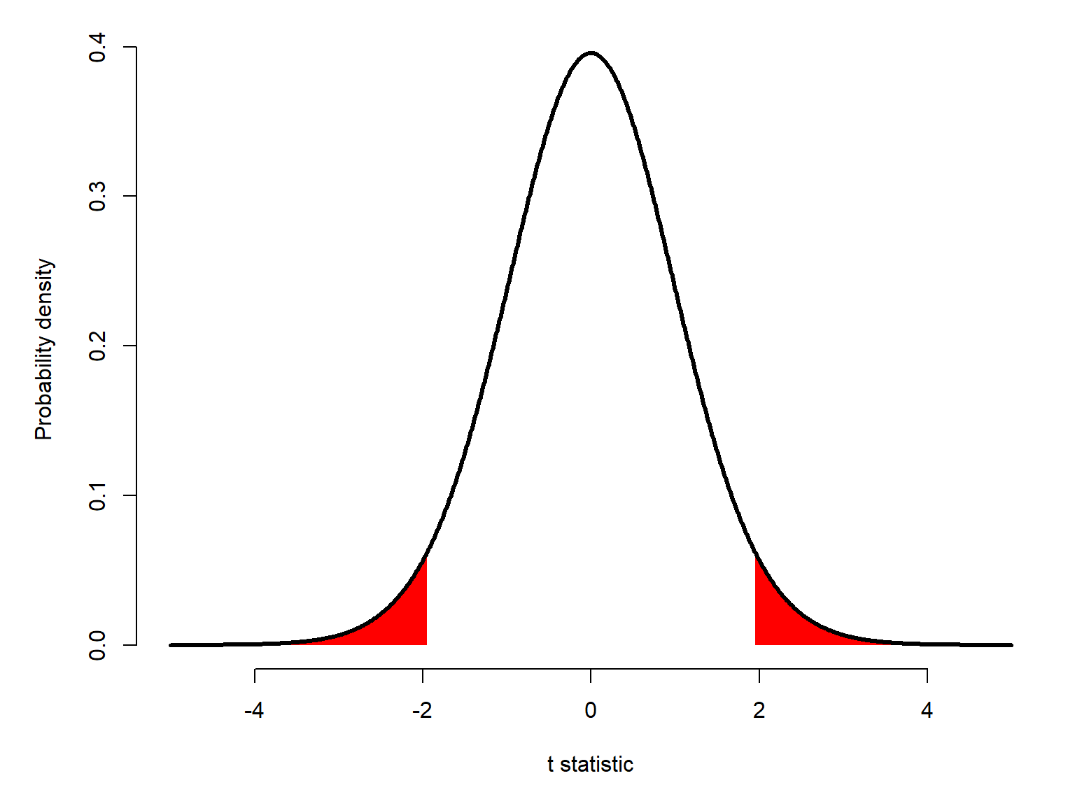
Say you perform a test comparing groups A and B, and the t statistic comes out to be 1.95. We have to compare that to the t distribution with the number of DF contained in the data, which might be 31.2:
The question for the hypothesis test is: in a dataset with 31.2 DF, how often should we observe t values at least as large as 1.95 (i.e., \(\left|t\right|\ge1.95\))? That proportion is the area shaded below:
The area of the left shaded area is pt(-1.95, 31.2), which is 0.0301. The distribution is symmetrical, so \(p\left(\left|t\right|\ge1.95\right)=0.0301\times2=0.0602\). Thus, the test was not significant (t = 1.95, 31.2 d.f., p = 0.06).
Question: Do two groups have the same underlying population mean?
Null hypothesis: The true difference in means = 0. I.e., \(\mu_1=\mu_2\).
Alternative hypothesis: True difference in means is \(\neq0\). I.e., \(\mu_1\neq\mu_2\).
Example use case: Barney needs to test whether tomato plants treated with a new pesticide have a different yield (g tomato / plant) than plants in the untreated control group.
Below is an example where we simulate some data and run a two-sample, two-tailed test to compare the means of two groups.
# simulate dataset.seed(42)a <-rnorm(100, 5, 2)b <-rnorm(100, 3, 2)# example 1: difference in meanst.test(a,b)
    Welch Two Sample t-test

data:  a and b
t = 8.1211, df = 194.18, p-value = 5.241e-14
alternative hypothesis: true difference in means is not equal to 0
95 percent confidence interval:
 1.696004 2.783990
sample estimates:
mean of x mean of y
 5.065030  2.825033
Interpretation: The researcher should conclude that there is a statistically significant difference between the means of groups a and b. In a manuscript, you should report the test statistic, the DF, and the p-value. E.g., “There was a significant difference in means between group a and group b (\(t=8.121\), 194.18 d.f., \(p<0.001\)).” Notice that values are rounded to 2 or 3 decimal places, which is usually enough for biology. This is especially true for the p-value, which can be approximated by R down to infinitesimally small values. I always round those to 0.001 or 0.0001.
A t-test can also be performed using the formula interface, which is an R programming construct for specifying a response variable and its predictors. Notice that the formula interface here is the same as used in boxplot() (Section 8.1.3) and aggregate() (Section 7.1.1).
Syntax note: Formula syntax has the response variable on the left, then a ~, then the predictor or predictors. For predictors, a + b means an additive model; while a * b specifies an interaction. For a t-test, there can be only 1 predictor. If you want to test \(>1\) predictor at a time, you need to use ANOVA instead.
Here are some common formula examples:
Table 15.1: Common R model formulas and their meanings.
Formula
Meaning
y ~ x
y is modeled as a function of x.
y ~ x1 + x2
y is modeled as a function of x1 and x2, with their effects treated as additive (i.e., no interaction between them is included).
y ~ x1 * x2
y is modeled as a function of x1, x2, and their interaction. An interaction means that the effect of one predictor depends on the value of the other predictor. This is shorthand for y~x1 + x2 + x1:x2.
y ~ 1
y is modeled using only a constant (the intercept), with no predictors. This is often called an intercept-only or null model.
y ~ 0 + x
y is modeled as a function of x, but without an intercept (i.e., the intercept is constrained to 0).
The formula interface is used in several contexts in R, including plotting, modeling, and aggregating.
# pull some data from example dataset iris# i.e., make a new data frame with only 2 groupsdx <- iris[which(iris$Species %in%c("setosa", "versicolor")),]# perform the test.t.test(Petal.Length~Species, data=dx)
    Welch Two Sample t-test

data:  Petal.Length by Species
t = -39.493, df = 62.14, p-value < 2.2e-16
alternative hypothesis: true difference in means between group setosa and group versicolor is not equal to 0
95 percent confidence interval:
 -2.939618 -2.656382
sample estimates:
    mean in group setosa mean in group versicolor
                   1.462                    4.260
Interpretation: The researcher should conclude that there is a statistically significant difference between the mean petal length of Iris setosa and Iris versicolor.
15.2.2 Two-sample, one-tailed t-tests
Question: Is the true difference in means between 2 groups greater than, or less than, some target value \(\mu\)?
Null hypothesis: The true difference in means between 2 groups is \(\mu\). I.e., \(\mu_1-\mu_2=\mu\).
Alternative hypothesis: The true difference in means between 2 groups is either greater than \(>\mu\) or \(<\mu\). I.e., either \(\mu_1-\mu_2>\mu\) or \(\mu_1-\mu_2<\mu\).
Example use case: Betty needs to compare two stock solutions and check that their pH differs by no more than 0.2.
The 2-sample, 1-tailed t-test that can be used in several ways:
Test whether the mean in one group is greater or less than the mean in another group.
Test whether the the mean in one group is greater or less than the mean in another group, and that the difference is at least some specified value.
For example, if you know that the mean of group 1 must be less than the mean in group 2, and will not even consider that the mean of group 2 is less than that of group 1, then you could run a 2-sample 1-tailed test.
    Welch Two Sample t-test

data:  x1 and x2
t = -8.8728, df = 37.99, p-value = 1
alternative hypothesis: true difference in means is greater than 0
95 percent confidence interval:
 -2.402592       Inf
sample estimates:
mean of x mean of y
 9.689982 11.708940
# is mean(x1) < mean(x2)?t.test(x1, x2, alternative="less")
    Welch Two Sample t-test

data:  x1 and x2
t = -8.8728, df = 37.99, p-value = 4.259e-11
alternative hypothesis: true difference in means is less than 0
95 percent confidence interval:
      -Inf -1.635323
sample estimates:
mean of x mean of y
 9.689982 11.708940
# is mean(x1) - mean(x2) at least 1?t.test(x1, x2, alternative="greater", mu=1)
    Welch Two Sample t-test

data:  x1 and x2
t = -13.267, df = 37.99, p-value = 1
alternative hypothesis: true difference in means is greater than 1
95 percent confidence interval:
 -2.402592       Inf
sample estimates:
mean of x mean of y
 9.689982 11.708940
# is mean(x1) - mean(x2) at most 1?t.test(x1, x2, alternative="less", mu=1)
    Welch Two Sample t-test

data:  x1 and x2
t = -13.267, df = 37.99, p-value = 3.867e-16
alternative hypothesis: true difference in means is less than 1
95 percent confidence interval:
      -Inf -1.635323
sample estimates:
mean of x mean of y
 9.689982 11.708940
an uncommon variant used to test whether two groups have a difference in means that is less than or greater than some specified value. For example, if you produce two batches of bacteria by inoculation, incubation, and then serial dilution, you may want to confirm that the difference in cell count between them is less than some acceptable value. You could use a 2-sample, 1-tailed test with the “alternative” hypothesis being that the difference is “greater” than your benchmark.
set.seed(789)x1 <-rnorm(30, 5, 2)x2 <-rnorm(30, 5.5, 2)# is the true difference in means <1?t.test(x1, x2, alternative="greater")
    Welch Two Sample t-test

data:  x1 and x2
t = -2.6676, df = 50.08, p-value = 0.9949
alternative hypothesis: true difference in means is greater than 0
95 percent confidence interval:
 -2.048126       Inf
sample estimates:
mean of x mean of y
 4.438104  5.696001
15.2.3 Equivalence testing
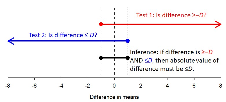
It is not possible to demonstrate statistically that a difference in means is truly 0, or that the underlying mean of a set of data truly is equal to a target value \(\mu\) (the converse of a one-sample, two-tailed t-test). With a 1-sample, 2-tailed test the best you can do is “fail to reject” the null hypothesis that the mean is 0. However, we can show that the difference is arbitrarily close to 0. This approach is called equivalence testing, and one method is the two one-sided tests (TOST) method. The method works like this:
Illustration of the two one-sided test (TOST) strategy for establishing that a sample, or set of differences, has an underlying mean arbitrarily close to some value \(\mu\) (\(\mu=0\) in this example.)
Here is a worked TOST equivalence test example in R:
# simulate dataset.seed(42)a <-rnorm(100, 5, 1)b <-rnorm(100, 5, 1)# let target tolerance = 1# note that total tolerance range is 1, so# amount for both one-sided tests is 1/2==0.5D <-0.5# test 1: is difference >-D?t.test(a, b, alternative ="greater", mu=-D)
    Welch Two Sample t-test

data:  a and b
t = 4.4956, df = 194.18, p-value = 5.955e-06
alternative hypothesis: true difference in means is greater than -0.5
95 percent confidence interval:
 -0.1079329        Inf
sample estimates:
mean of x mean of y
 5.032515  4.912516
# test 2: is difference <D?t.test(a, b, alternative ="less", mu=D)
    Welch Two Sample t-test

data:  a and b
t = -2.7554, df = 194.18, p-value = 0.00321
alternative hypothesis: true difference in means is less than 0.5
95 percent confidence interval:
    -Inf 0.34793
sample estimates:
mean of x mean of y
 5.032515  4.912516
Interpretation: Test 1 showed that the difference in means is \(>-0.5\). Test 2 showed that the difference in means is \(<0.5\). So, the difference in means is in the interval \(\left(-0.5,0.5\right)\), which means the difference in means is at most 0.5 in either direction.
15.2.4 Wilcoxon rank-sum test
Question: Are values in one group consistently greater than or less than those in another group? OR: Is the median rank in one group different from that in another group?
Null hypothesis: For randomly selected values \(x\) and \(y\) from two groups, \(p\left(x>y\right)=p\left(y>x\right)\).
Alternative hypothesis: For randomly selected values X and Y from two groups, \(p\left(x>y\right)\neq p\left(y>x\right)\).
Example use case: Homer is interested in whether plots where invasive plants have been removed have more squirrels than plots where invasive plants are not removed, but does not want to model the actual number of squirrels.
The Mann-Whitney U test, also known as the Wilcoxon test, is a nonparametric alternative to the two-sample t-test. Nonparametric means that the test does not make restrictive assumptions about the distribution of the data or a test statistic. Nonparametric tests are often based on the ranks of the data: the smallest value is rank 1, the next smallest is rank 2, and so on. Because of this, nonparametric tests allow you make statements about how consistent a pattern is, rather than about the actual values.
This test has two common use cases:
The researcher is only interested in whether values in one group are consistently larger than those in another group.
The researcher needs to perform a t-test, but the data do not meet the assumptions of the t-test.
The syntax for the Wilcoxon test is fairly similar to that of a t-test.
Example Wilcoxon test in R:
# simulate some data:set.seed(123)a <-runif(20, 1, 6)b <-runif(20, 4, 9)# run the testwilcox.test(a,b)
    Wilcoxon rank sum exact test

data:  a and b
W = 35, p-value = 1.126e-06
alternative hypothesis: true location shift is not equal to 0
Here is the same kind of test, but using the formula interface. You can use the formula interface for t-tests as well.
# pull some data from example dataset iris# i.e., make a new data frame with only 2 groupsuse.species <-c("versicolor", "virginica")dx <- iris[which(iris$Species %in% use.species),]dx$Species <-factor(dx$Species, levels=use.species)# perform the test.wilcox.test(Petal.Length~Species, data=dx)
    Wilcoxon rank sum test with continuity correction

data:  Petal.Length by Species
W = 44.5, p-value < 2.2e-16
alternative hypothesis: true location shift is not equal to 0
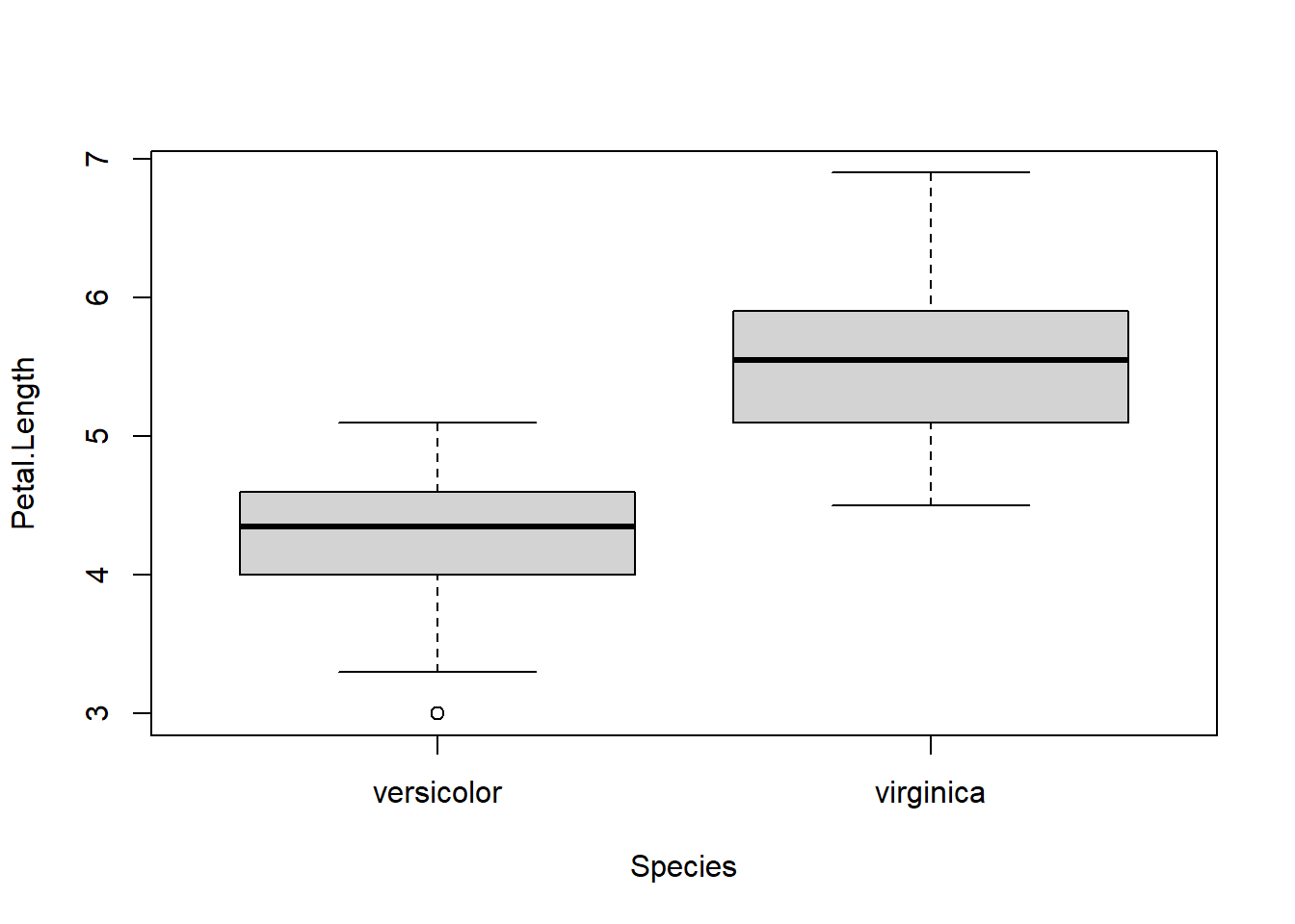
Interpretation: The researcher can say that values in one group are consistently greater than values in the other group. Which way that goes should be obvious from looking at the sample medians or a boxplot.
# follow up the test with a boxplot# note that the formula interface is used here as well!boxplot(Petal.Length~Species, data=dx)
When sample sizes or effect sizes are large, the Wilcoxon test and the t-test will often give the same answers in terms of significance vs. nonsignificance.
Because the t-test tests for a difference in means, and the Wilcoxon is its rank-based alternative, some people think that the Wilcoxon test is a test for a difference in medians…but this is not correct. It’s more accurate to say that the Wilcoxon test tests for a median difference.
15.3 Tests for paired data
15.3.1 Paired t-test
Question: Is the mean of the differences of paired observations = 0, or different from 0?
Null hypothesis: Mean of pairwise differences = 0.
Alternative hypothesis: Mean of pairwise differences \(\neq0\).
Example use case: Pebbles needs to test for a mean change in the body mass of individual mice before and after a feeding trial. Each mouse is weighed both before and after the trial.
Many biological experiments involved paired samples, where a single unit or entity was measured twice. For example, a single mouse might be weighed before and after a feeding trial. In a paired t-test, we test whether or not the mean of differences is 0. This is subtly different than the test for differences in means evaluated in a two-sample test. Consequently, a paired t-test is tantamount to a one-sample test on the pairwise differences. Compare the null hypotheses tested by the two-sample t-test and paired t-test below:
Let’s simulate some data, conduct a paired t-test, and convince ourselves that the paired t-test is equivalent to a one-sample test on pairwise differences.
# Example paired t-test in R# simulate dataset.seed(42)a <-rnorm(100, 5, 2)# add pair-wise differencesb <- a +rnorm(100, 2, 0.2)
Interpretation: The researcher should conclude that the mean difference for each subject was significantly different from 0, at -1.98 with a 95% CI of [-2.02, -1.95].
Note that the paired t-test gives essentially the same result as conducting a one-sample test on the pair-wise differences.
# compare to one sample t-test on differences:dif <- b - at.test(dif)
    One Sample t-test

data:  dif
t = 109.63, df = 99, p-value < 2.2e-16
alternative hypothesis: true mean is not equal to 0
95 percent confidence interval:
 1.946622 2.018385
sample estimates:
mean of x
 1.982503
15.4t-test summary
As we have seen, the t-test in all of its variations is a very useful and flexible family of tests that can be applied to many biological problems. One of the reasons that t-tests are so widely applicable-and why there are so many t-tests–is that the test statistic t is so elegant in its construction: it represents the quantity of interest directly in its numerator, and then the denominator scales that quantity according to the level of uncertainty in the data. It is thus a kind of signal-to-noise ratio that predated information theory by almost 50 years.
As a review, the table below summarizes the different t-tests and their use cases:
Table 15.2: Common types of t-tests and the hypotheses they evaluate.
Type
Use
Section
One-sample t-test, one-tailed
Tests whether the population mean of a single set of values is less than or greater than a specified value \(\mu_0\). Appropriate when differences in only one direction are of interest.
Tests whether the population means of two groups (\(\mu_1\) and \(\mu_2\)) differ. This can also be thought of as testing whether the difference between the means is equal to 0. Welch’s t-test, which does not assume equal variances, should generally be used and is the default in R.
Tests whether the population mean of one group (\(\mu_1\)) is less than or greater than the mean of another group (\(\mu_2\)). Appropriate when differences in only one direction are of interest.
Tests whether the mean difference between paired observations differs from a specified value \(D_0\), usually 0. The test may be one- or two-tailed depending on the hypothesis.
The number of “samples” in a t-test refers to how many sets of observations are being compared. There can be either 1 sample (all observations compared to some value) or 2 samples (2 sets of observations compared to each other).
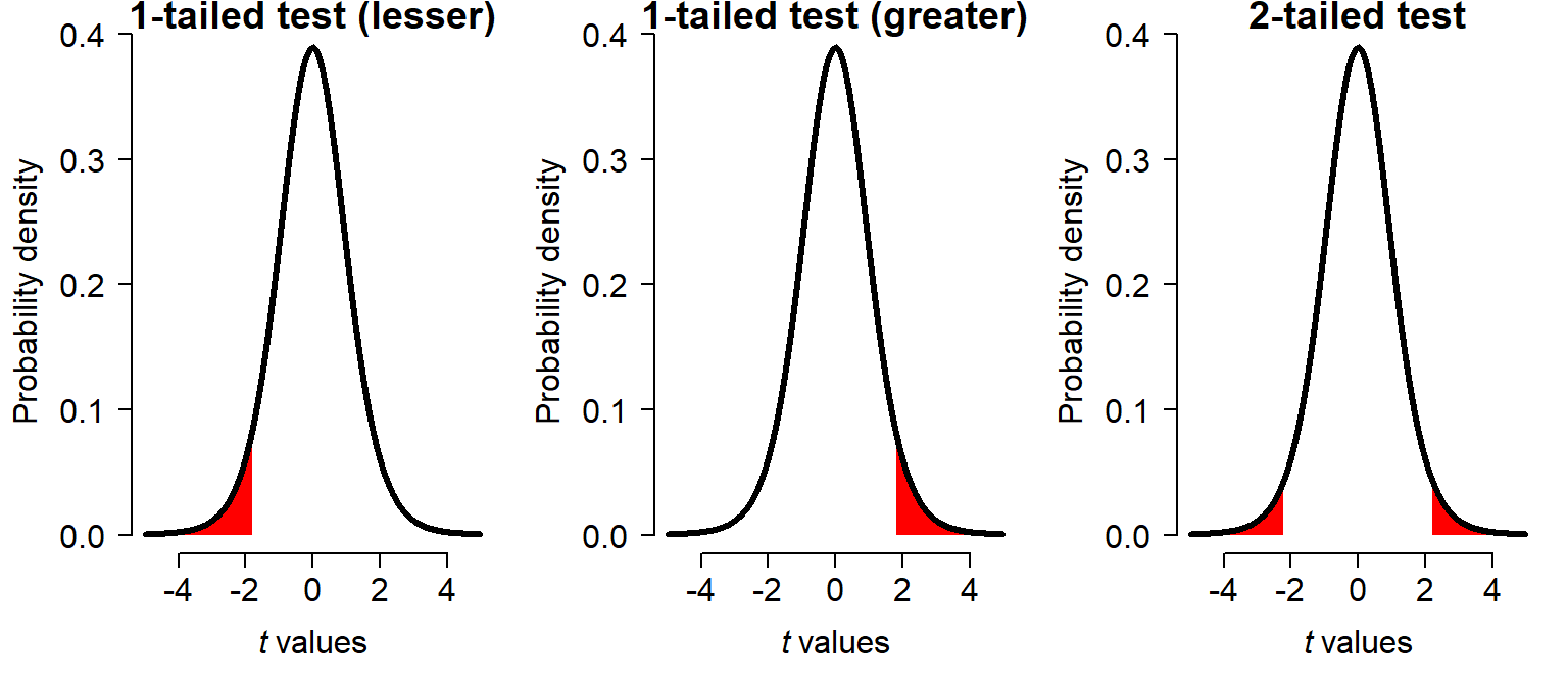
The number of “tails” refers to how sides (left (negative) and/or right (positive)) are of interest in the test statistic distribution. In a two-tailed test, or two-sided test, an extreme test statistic could fall in either the right or the left tail of the distribution. The figure below shows the range of t values which would be declared significant for each kind of test. Notice that for a one-tailed test, the significance region extends closer to the center, because its area must be equal to the same \(\alpha\) as a two-tailed test.
The t-test is usually one of the first methods taught because its use cases are simple, and its test statistic is pretty easy to understand. Consider the original t statistic introduced to the English statistics literature by Gosset and popularized as “Student’s t” by Fisher:
The numerator is the quantity of interest: the difference in sample means. It should make sense that the larger the difference in sample means, the greater the probability that the difference will be statistically significant. However, considering only the sample means \(\bar{x_1}\) and \(\bar{x_2}\) is not enough. We also need to account for variation within each sample, and for the total sample size. Variance should decreaset, while sample size should increase it. Both terms are put in the denominator so that the difference in means is relative to them. Notice that in the denominator, the variances \(s_{x_1}^1\) and \(s_{x_2}^1\) are in a numerator. Thus, increasing them will decrease t. On the other hand, the sample size n is in a numerator in the denominator (which is tantamount to being in the overall numerator). Thus, increasing sample size will increase t.
But as elegant as Student’s t is, it has some drawbacks. It can produce biased estimates and p-values when the two groups have unqual sample sizes, or unequal variances. For these reasons, a more modern version of the t statistic was developed by Welch in the 1940s. This is sometimes called the “Welch’s t-test”, or less precisely the “Welch-Satterthwaite t-test”. Satterthwaite’s contribution was not to the t statistic, but rather an equation to better calculate the degrees of freedom to use for the test2.
\[
t=\frac{\bar{x_1}-\bar{x_2}}{\sqrt{\frac{s_1}{\sqrt{n_1}}+\frac{s_2}{\sqrt{n2}}}}
\] This newer version has the same numerator, but instead of pooling the variances and sample sizes, keeps them separate. This allows for more flexibility when dealing with unequal sample sizes or (mildly) heteroscedastic data.
15.5 Tests for 3 or more groups
15.5.1 Analysis of variance
In this section, we will explore the “test comparing group means” sense of analysis of variance (ANOVA) (Section 14.5). The linear model version of ANOVA assesses significance using an F-test. Much like t, F is a test statistic that summarizes a quantity of interest in a test that can be compared to the typical strength of a pattern produced by random noise (see Section 15.2.1}). Whereas t is usually a difference in means scaled by sample size and variance, F compares variances. The basic idea of an F statistic is:
where \(\bar{Y}_{i}\) is the sample mean in group \(i\), \(n_i\) is the number of observations in group \(i\), \(\bar{Y}\) is the overall mean of the data, and \(K\) is the number of groups.
The denominator is close to the the sum of within-group variances:
where \(Y_{ij}\) is observation \(j\) in group \(i\) (out of \(K\) groups), and \(N\) is the overall sample size.
The \(F\) statistic is a ratio of variance explained to variance not explained. F values follow the F distribution, which is defined by degrees of freedom \(d_1=K-1\) and \(d_2=N-K\) under the null hypothesis. Practically, F will be large when there is more explained variance than unexplained variance, which is unlikely if the group means are not different.
Question: Do the means differ between groups (with number of groups \(\geq2\).
Null hypothesis: All group means are equal.
Alternative hypothesis: At least one group mean is different from the others.
Example use case: Marge needs to test whether cucumber mass is greater in plants grown in potting mix, sandy soil, or clayey soil.
The nature of the F statistic belies the other meaning of ANOVA: the partitioning of variation into its different sources. In other words, what proportion of variation in the Y variable does each factor explain? How much variation is due to random chance (i.e., residual variation)? ANOVA in this sense can be applied to many models, including all linear models.
The first step in a typical ANOVA is the omnibus test, which assesses whether any of the group means differ from each other. Then, a post-hoc test is performed to check which groups differ from each other.
ANOVAs are typically described as “X-way ANOVA”, where X is the number of factors. For example, a test of mean stomach size in herbivorous, carnivorous, and omnivorous mammals would be a “one-way ANOVA” because it has one grouping variable, “diet”. The three groups in the factor diet are the levels of the factor.
15.5.1.1 One-way ANOVA
When there is one explanatory factor, or grouping variable, the test is called a one-way ANOVA regardless of how many levels or groups that factor contains. Here is an example using the built-in example dataset iris. There are two common ways to fit an ANOVA in R.
Once the model is fit, we request the anova table so we can see the contributions of each source of variation.
# method 1: using lmanova(mod1)
Analysis of Variance Table

Response: Petal.Length
           Df Sum Sq Mean Sq F value    Pr(>F)
Species     2 437.10 218.551  1180.2 < 2.2e-16 ***
Residuals 147  27.22   0.185
---
Signif. codes:  0 '***' 0.001 '**' 0.01 '*' 0.05 '.' 0.1 ' ' 1
# method 2: using aovsummary(mod2)
             Df Sum Sq Mean Sq F value Pr(>F)
Species       2  437.1  218.55    1180 <2e-16 ***
Residuals   147   27.2    0.19
---
Signif. codes:  0 '***' 0.001 '**' 0.01 '*' 0.05 '.' 0.1 ' ' 1
No matter which method we use, the ANOVA table shows us that the factor Species uses 2 degrees of freedom (variously abbreviated as DF, Df, or d.f.) to account for 437.10 of the squared errors; the residuals use 147 d.f. to account for 27.22 of the squared errors. The ratio of the mean squared error per d.f. associated with each source, 218.551 / 0.185 = 1180.2, is the test statistic F. This is used to calculate the P-value (much like t, F follows a particular distribution defined by DF, which allows \(p(F)\) to be calculated). We can also see that about 94.1% of variation (437.10 / (437.10+27.22)) is associated with species. This is the model’s coefficient of determination, or \(R^2\). The \(R^2\) tells you the proportion of variation in Y explained by the model.
Tip
Rounding errors
R is somewhat idiosyncratic in choosing how many digits it prints, and this can lead to confusion if values are rounded to too few decimal places. In the ANOVA example above, the MSE for the two sources of variation should divide to the F statistic. However, \(218.55/0.19\neq1180\). If you look at the raw output of mod1, however, you that the sums of squares for Species and Residuals are 437.1028 and 27.2226, respectively. With more decimal places, you can then recalculate \(\left(437.1028/2\right)/\left(27.2226/147\right)=1180.161\), the correct \(F\) ratio.
Remember that the all that the omnibus test p-value tells you is that the means of at least one pair of species differ. To find out which pair or pairs, we need to use a post-hoc test. My favorite is the Tukey’s honest significant difference (HSD) test because it automatically adjusts for multiple comparisons.
  Tukey multiple comparisons of means
    95% family-wise confidence level

Fit: aov(formula = Petal.Length ~ Species, data = iris)

$Species
                      diff     lwr     upr p adj
versicolor-setosa    2.798 2.59422 3.00178     0
virginica-setosa     4.090 3.88622 4.29378     0
virginica-versicolor 1.292 1.08822 1.49578     0
The Tukey output shows us that every group differs from every other, with p<0.001 (here p is rounded to 0, although it can never be 0). The differences in group means are presented with their 95% confidence intervals (CI). For example, the difference between the group means of versicolor and setosa is 2.798 cm, with 95% CI = [2.594, 3.002]. The fact that the difference is \(>0\) means that the mean in versicolor is greater than the mean in setosa. If the difference was negative, then that would mean that the mean in setosa was greater.
Notice that none of these CI include 0: this suggests that a true difference of 0 between any two groups is very unlikely. Even without examining p-values, CI provide a useful way to evaluate both the direction and magnitude of differences.
One of the nice things about the Tukey HSD test is that the p-values are automatically adjusted for multiple comparisons, a phenomenon where the probability of a false positive goes up as a researcher performs more tests, using a customized version of the probability distribution for the test statistic. This controls the family wise error rate, or total false positive probability for this set of three related tests.
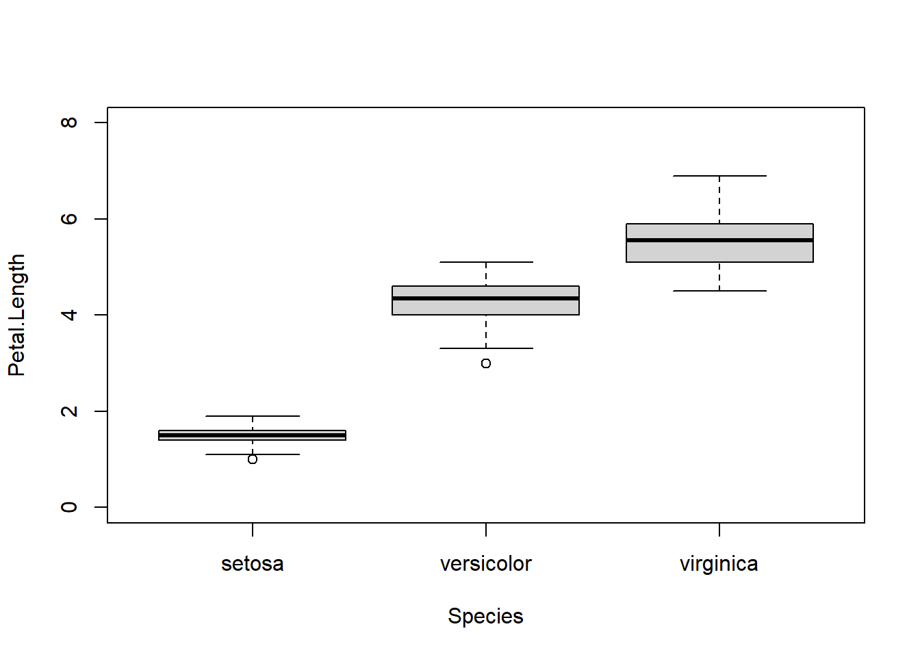
As with a t-test, a boxplot is usually the best way to show the results of an ANOVA.
Figure 15.1: Boxplot showing that petal length is greater in Iris versicolor than in Iris setosa, and greater still in Iris virginica.
15.5.1.2 Two- or more way ANOVA
When there are 2 or more explanatory factors, the test is called a two-way ANOVA, or three-way ANOVA, and so on. We can add additional factors to an ANOVA with the + sign.
# make a copy of iris with an extra grouping variableiris2 <- irisiris2$Flower <-c("purple", "pink")# fit the two-way ANOVA without interactionmod3 <-aov(Petal.Length~Species+Flower, data=iris2)summary(mod3)
             Df Sum Sq Mean Sq  F value Pr(>F)
Species       2  437.1  218.55 1174.229 <2e-16 ***
Flower        1    0.0    0.05    0.261   0.61
Residuals   146   27.2    0.19
---
Signif. codes:  0 '***' 0.001 '**' 0.01 '*' 0.05 '.' 0.1 ' ' 1
Adding the colors that way just repeated them until the column was full: purple, pink, purple, pink, and so on until the new vector had length 150 (the number of rows in iris). This essentially distributes the colors randomly with respect to the species and thus the petal lengths, so it should be no surprise that flower color had no effect on petal length (\(p=0.61\)). A Tukey test confirms the effects of species, and the non-effect of Flower. Technically, you don’t need to do or report a Tukey test if the main effect is nonsignificant.
TukeyHSD(mod3)
  Tukey multiple comparisons of means
    95% family-wise confidence level

Fit: aov(formula = Petal.Length ~ Species + Flower, data = iris2)

$Species
                      diff      lwr      upr p adj
versicolor-setosa    2.798 2.593692 3.002308     0
virginica-setosa     4.090 3.885692 4.294308     0
virginica-versicolor 1.292 1.087692 1.496308     0

$Flower
             diff        lwr       upr     p adj
purple-pink 0.036 -0.1032347 0.1752347 0.6101255
15.5.1.3 ANOVA with interaction
Another important question is whether there is an interaction between two variables. An interaction is a situation where one variable changes the effect of another. To test for an interaction between two variables, use the * symbol instead of the +. The result y~x1*x2 is shorthand for y~x1+x2+x1:x2. The individual effects of the variables x1 and x2 are called their main effects. The effect of both together x1:x2 is the interaction effect. If a significant interaction effect is detected, then the main effects should not be interpreted by themselves.
# fit the two-way ANOVA WITH interactionmod3 <-aov(Petal.Length~Species*Flower, data=iris2)summary(mod3)
                Df Sum Sq Mean Sq  F value Pr(>F)
Species          2  437.1  218.55 1161.375 <2e-16 ***
Flower           1    0.0    0.05    0.258  0.612
Species:Flower   2    0.1    0.04    0.201  0.818
Residuals      144   27.1    0.19
---
Signif. codes:  0 '***' 0.001 '**' 0.01 '*' 0.05 '.' 0.1 ' ' 1
The interaction is nonsignificant, so we should instead report the main effects in the model without the interaction (mod2). If there is an interaction present, then it becomes impossible to discuss the effects of one variable without discussing the effects of the other. We will explore interactions more in the section on ANCOVA below.
15.5.1.4 Blocking designs
Blocking is a strategy in experimental design that attempts to control for variation by grouping experimental units (observations) into groups called blocks. Blocks are defined by observations that are similar to each other in some attribute–like location, time, sex, species, etc.–that contributes to overall variation and that the researcher needs to control for.
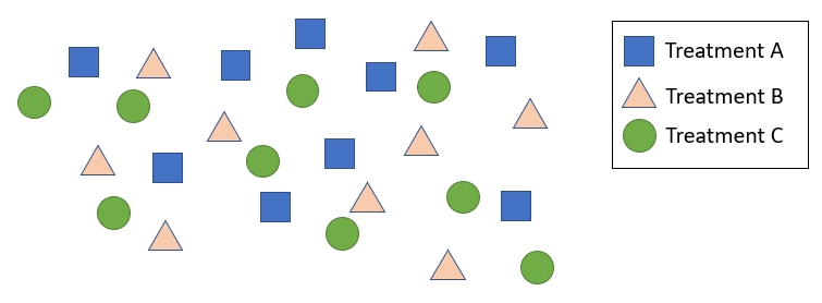
Consider the example below.
Illustration of a field experiment with 3 researcher-applied treatments, A, B, and C, spread out over a landscape.
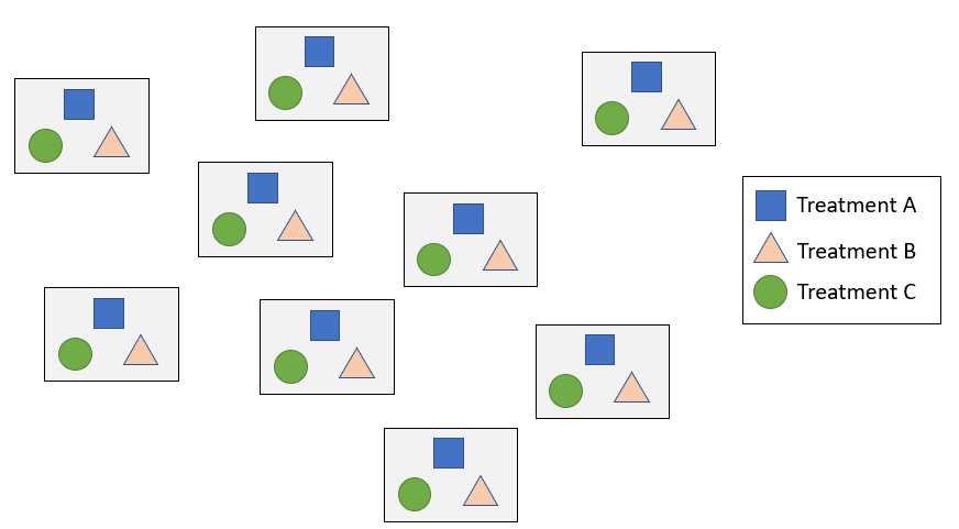
This experiment appears to have randomly distributed its treatments across space, which is good. However, there will still be variation among observations that is caused by different environments or habitats in different places. Rather than model those location-specific differences explicitly, the research could instead distributed blocks of observations randomly across space, with each block containing 1 observation of each of the 3 treatments.
{fig-alt=“fig-alt=”Schematic of a blocked experimental design with three treatments. Experimental units assigned to Treatment A, Treatment B, and Treatment C are represented by blue squares, orange triangles, and green circles, respectively. The units are arranged into nine blocks, shown as rectangles, with each block containing one unit from each treatment.”}
Now, variation attributable to spatial factors can be associated with the blocks and no longer confounds the effects of treatment. Observations within a block should be close enough that they experience the same environmental conditions.
In the example code below, we are going to add an imaginary factor to the iris dataset, color. The example analysis shows how a researcher would test for a difference in petal length between flowers of different colors, while accounting for the fact that different species have different petal lengths. In this analysis, the researcher is interested in differences between colors, and considers species a potential confounding variable.
This example works because we force the color effect with an artificial variable, and because the setup says explicitly that the researcher considers species a potential confound. From an experimental design standpoint, blocking is not synonymous with “a second categorical factor in an ANOVA”, although that is how it is treated mathematically.
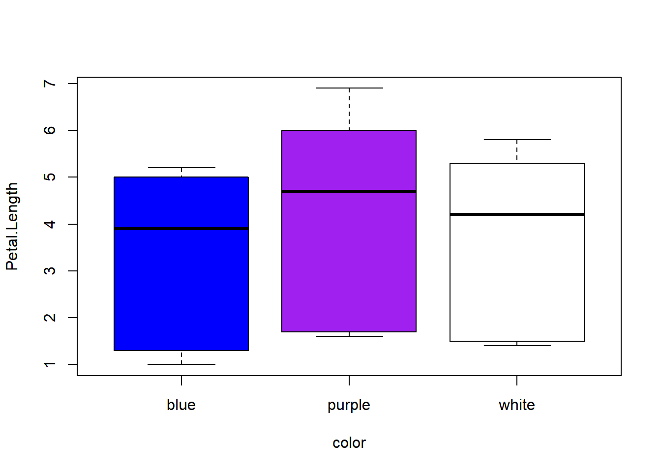
# spare copydx <- iris# make the largest flowers within each species purple,# and the smallest flowers blue. # scale within speciesz <-tapply(dx$Petal.Length, dx$Species, scale)dx$z <-do.call(c, z)# any flower >= 0.6 SD away from mean# is a non-white colordx$color <-"white"dx$color[which(dx$z <=-0.6)] <-"blue"dx$color[which(dx$z >=0.6)] <-"purple"# vector of colorscols <-c("blue", "purple", "white")boxplot(Petal.Length~color, data=dx, col=cols)
The boxplot shows that the sample medians for blue, white, and purple are the smallest, intermediate, and greatest, respectively. But is that a significant difference?
# test for effect of color on petal lengthsummary(aov(Petal.Length~color, data=dx))
             Df Sum Sq Mean Sq F value Pr(>F)
color         2   13.6   6.805   2.219  0.112
Residuals   147  450.7   3.066
No, it’s not. But at this point the researcher should suspect that a lot of variation is size is really due to species. If she controls for species by treating it as a blocking factor, then she might be better able to detect an effect of color.
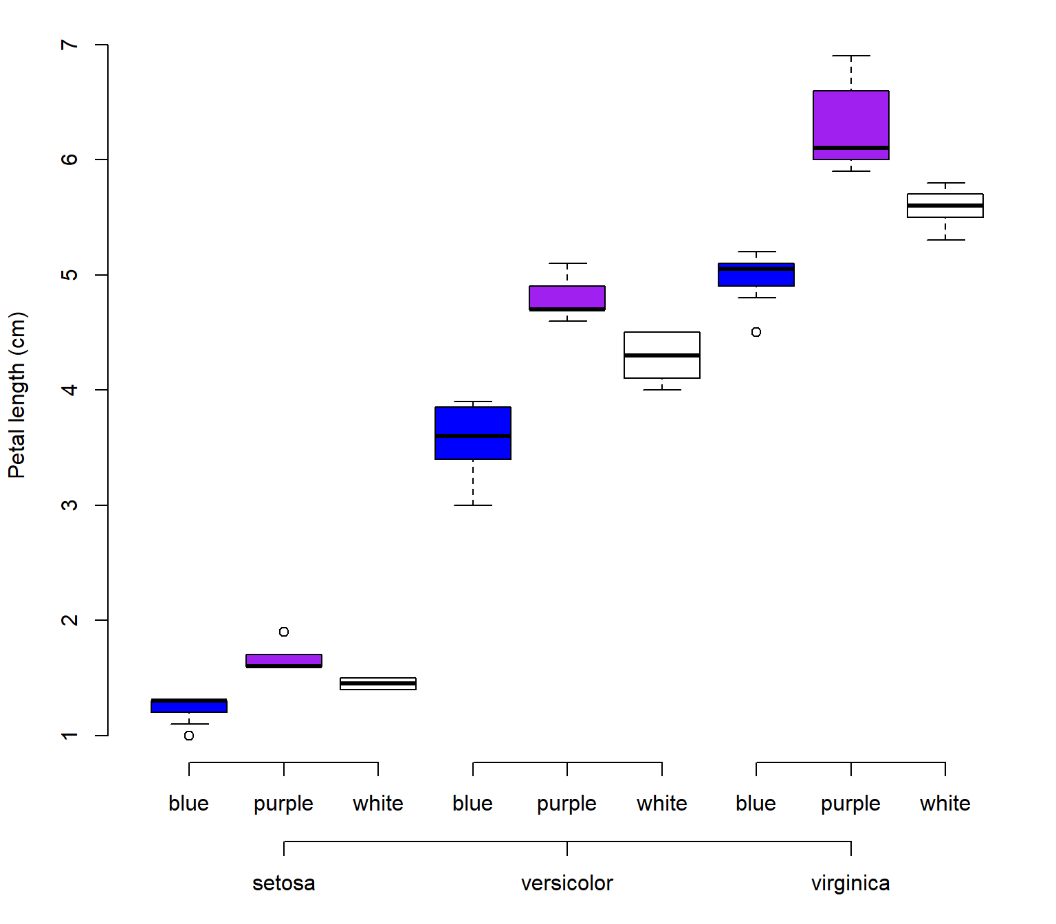
Below is the same petal length data broken up by color within species. Now, we can see that within each species, blue flowers are smaller and purple flower are larger. The first ANOVA couldn’t detect that because it didn’t consider species.
Also, note the use of axis() to create a more elegant set of labels for the x-axis.
             Df Sum Sq Mean Sq F value Pr(>F)
color         2   13.6    6.81   130.6 <2e-16 ***
Species       2  443.2  221.58  4251.0 <2e-16 ***
Residuals   145    7.6    0.05
---
Signif. codes:  0 '***' 0.001 '**' 0.01 '*' 0.05 '.' 0.1 ' ' 1
This shows that there is a significant effect of color, after species has been accounted for. We can also see why species covered the effect of color: there are considerably more sums of squares associated with species than with color.
anovatable[[1]][,2]/sum(anovatable[[1]][,2])
[1] 0.02931143 0.95441113 0.01627743
The total variance is approximately \(13.61+443.16+7.56=464.33\). Most of that variance (\(100\left(443.16/464.33\right)\approx95.4\%\)) is attributed to differences between species. Only about 3% (\(13.61/464.33\)) is attributed to color. It’s a small effect, but a significant one, and only detectable after accounting for species.
15.5.1.5 Repeated measures ANOVA
Coming soon!
15.5.2 Kruskal-Wallis test
Question: Are values in one or more groups consistently greater or less than values in another group? (number of groups \(\geq3\)); essentially extends Wilcoxon test to more groups)
Null hypothesis: For randomly selected values \(x\) and \(y\) from any 2 groups, \(p\left(x>y\right)=p\left(y>x\right)\).
Alternative hypothesis: For randomly selected values \(x\) and \(y\) from any 2 groups, \(p\left(x>y\right)\neq p\left(y>x\right)\)
Example use case: Bart is studying whether tomato yields tend to be greater in plants treated with no pesticide, pesticide A, or pesticide B. He is not interested in predicting the actual tomato yield.
Because ANOVA is a linear model, the data used in ANOVA must meet the assumptions of the linear model. If the data do not meet the assumptions, or cannot be transformed to do so, then a nonparametric alternative to ANOVA is needed. The most common alternative is the Kruskal-Wallis test. Some texts refer to this as a “nonparametric ANOVA”, but this is not correct because at no point is variance actually partitioned. Like the Wilcoxon test, the Kruskal-Wallis test is based on ranks of the data. A significant Kruskal-Wallis test indicates that values in at least one group are consistently greater than values in at least one other group. As with ANOVA, a post-hoc test is needed to determine which groups differ significantly from each other.
Example Kruskal-Wallis test in R
kruskal.test(Petal.Length~Species, data=iris)
    Kruskal-Wallis rank sum test

data:  Petal.Length by Species
Kruskal-Wallis chi-squared = 130.41, df = 2, p-value < 2.2e-16
The significant result means that petal length is consistently greater for at least species compared to the other. This is analogous to the omnibus ANOVA test. If we want to know which groups differ, we need a post-hoc test. The most common option is the Dunn’s test.
  Kruskal-Wallis rank sum test

data: x and group
Kruskal-Wallis chi-squared = 130.411, df = 2, p-value = 0

                           Comparison of x by group
                                 (Bonferroni)
Col Mean-|
Row Mean |     setosa   versicol
---------+----------------------
versicol |  -5.862996
         |    0.0000*
         |
virginic |  -11.41838  -5.555388
         |    0.0000*    0.0000*

alpha = 0.05
Reject Ho if p <= alpha/2
Interpretation: A posthoc Dunn’s test showed that all three species differed from each other in terms of the rank order of petal lengths.
15.6 Tests with ordered factors
Some factors can represent group membership, but still have an inherent ordering to them. For example, soft drinks come in sizes “small”, “medium”, and “large”. These are categories, but categories in order: small < medium < large. In contrast, the three species in the iris dataset have no ordering.
You may have data with a factor for age, like “juvenile”, “subadult”, “adult”. These categories correspond to ages, but cannot be treated as literal numbers of years or months. It would also be a mistake to treat the comparison of “juvenile vs. subadult” the same as the comparison of “juvenile vs. adult”.
If you analyze an ordered factor, R will estimate polynomial terms of order up to \(k-1\), where \(k\) is the number of factor levels. The polynomial function is a way to fit different patterns across the ordered levels. For example, a linear pattern captures a monotonic increase or decrease across the levels. A quadratic pattern can describe a situation where the middle of three levels has greater (or smaller) values than the first and third levels. Let’s create a toy dataset to illustrate working with an ordered factor.
ages <-c("juvenile", "subadult", "adult")dx <-data.frame(age=rep(ages, each=20))# tell R that this is an ordered factordx$age <-factor(dx$age, levels=ages, ordered=TRUE)# notice the levels statement:dx$age
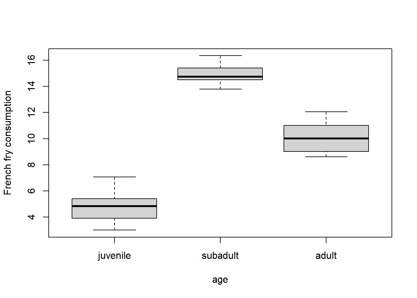
Figure 15.2: Boxplot showing that french fry consumption is greatest in subadults, less in adults, and lowest in juveniles.
Now fit the model using the ordered factor age:
mod11 <-aov(ff~age, data=dx)summary(mod11)
            Df Sum Sq Mean Sq F value Pr(>F)
age          2 1008.8   504.4   526.2 <2e-16 ***
Residuals   57   54.6     1.0
---
Signif. codes:  0 '***' 0.001 '**' 0.01 '*' 0.05 '.' 0.1 ' ' 1
The omnibus test shows us that age is significant. However, because we have an ordered factor, we don’t want something like a Tukey test. Group means are not of interest; rather, the pattern in group means across groups is. So, we what we want is to see which patterns across age are significant.
summary.lm(mod11)
Call:
aov(formula = ff ~ age, data = dx)

Residuals:
     Min       1Q   Median       3Q      Max
-1.88500 -0.78190 -0.08528  0.59410  2.17546

Coefficients:
            Estimate Std. Error t value Pr(>|t|)
(Intercept)   9.9419     0.1264   78.66   <2e-16 ***
age.L         3.6275     0.2189   16.57   <2e-16 ***
age.Q        -6.1060     0.2189  -27.89   <2e-16 ***
---
Signif. codes:  0 '***' 0.001 '**' 0.01 '*' 0.05 '.' 0.1 ' ' 1

Residual standard error: 0.9791 on 57 degrees of freedom
Multiple R-squared:  0.9486,    Adjusted R-squared:  0.9468
F-statistic: 526.2 on 2 and 57 DF,  p-value: < 2.2e-16
The coefficients for age.L and age.Q are the linear and quadratic trends, respectively. In this case, there is a positive linear trend (3.5113), so \(Y\) generally increases with age category. There is also a significant negative quadratic trend (-6.2328), meaning that the relationship is curved. These trends describe the shape of the trend with respect to the age categories, not literally the values of \(Y\) given \(X\) (as in a polynomial equation), so you need to inspect the boxplot or a plot of means.
This analysis was simple because there were only 3 levels of age. When an ordered factor has many levels, you may observe “significant” polynomial trends that are biologically unimportant or difficult to interpret. It is up to you as a biologist to exercise some judgement in deciding how many terms to interpret. For example, a quadratic pattern can be readily interpreted biologically. But what about a quintic? Or an octic?
Gosset published his work under the pen name “Student” because his employer at the time, the Guinness Brewery, didn’t want their competitors to know that they used the t-test in their quality control procedures.↩︎
This is why t-tests in R often report non-integer degrees of freedom.↩︎
 {fig-alt=“fig-alt=”Schematic of a blocked experimental design with three treatments. Experimental units assigned to Treatment A, Treatment B, and Treatment C are represented by blue squares, orange triangles, and green circles, respectively. The units are arranged into nine blocks, shown as rectangles, with each block containing one unit from each treatment.”}